Tr1: Differential Gene Expression

Last updated: 2023-05-02

Checks: 6 1

Knit directory: Tr1-RNA-Sequencing-/

This reproducible R Markdown analysis was created with workflowr (version 1.7.0). The Checks tab describes the reproducibility checks that were applied when the results were created. The Past versions tab lists the development history.

R Markdown file: uncommitted changes

The R Markdown file has unstaged changes. To know which version of the R Markdown file created these results, you’ll want to first commit it to the Git repo. If you’re still working on the analysis, you can ignore this warning. When you’re finished, you can run wflow_publish to commit the R Markdown file and build the HTML.

Environment: empty

Great job! The global environment was empty. Objects defined in the global environment can affect the analysis in your R Markdown file in unknown ways. For reproduciblity it’s best to always run the code in an empty environment.

Seed: set.seed(20221025)

The command set.seed(20221025) was run prior to running the code in the R Markdown file. Setting a seed ensures that any results that rely on randomness, e.g. subsampling or permutations, are reproducible.

Session information: recorded

Great job! Recording the operating system, R version, and package versions is critical for reproducibility.

Cache: none

Nice! There were no cached chunks for this analysis, so you can be confident that you successfully produced the results during this run.

File paths: relative

Great job! Using relative paths to the files within your workflowr project makes it easier to run your code on other machines.

Repository version: fa49ee5

Great! You are using Git for version control. Tracking code development and connecting the code version to the results is critical for reproducibility.

The results in this page were generated with repository version fa49ee5. See the Past versions tab to see a history of the changes made to the R Markdown and HTML files.

Note that you need to be careful to ensure that all relevant files for the analysis have been committed to Git prior to generating the results (you can use wflow_publish or wflow_git_commit). workflowr only checks the R Markdown file, but you know if there are other scripts or data files that it depends on. Below is the status of the Git repository when the results were generated:


Ignored files:
    Ignored:    .Rhistory
    Ignored:    .Rproj.user/

Unstaged changes:
    Conflicted: analysis/dge.Rmd

Note that any generated files, e.g. HTML, png, CSS, etc., are not included in this status report because it is ok for generated content to have uncommitted changes.

These are the previous versions of the repository in which changes were made to the R Markdown (analysis/dge.Rmd) and HTML (docs/dge.html) files. If you’ve configured a remote Git repository (see ?wflow_git_remote), click on the hyperlinks in the table below to view the files as they were in that past version.

File	Version	Author	Date	Message
Rmd	fa49ee5	Stevie Ped	2023-05-02	Removed grouping annotations from high_conf heatmap
html	fa49ee5	Stevie Ped	2023-05-02	Removed grouping annotations from high_conf heatmap
Rmd	ef7ce0c	Stevie Ped	2023-05-01	Made fonts larger. Not sure it was enough
html	ef7ce0c	Stevie Ped	2023-05-01	Made fonts larger. Not sure it was enough
html	63a6ba6	steveped	2022-11-24	Updated all figures
Rmd	39f0b04	Steve Pederson	2022-11-24	Added UpSet plot & heatmap of signatures
html	39f0b04	Steve Pederson	2022-11-24	Added UpSet plot & heatmap of signatures
Rmd	335d9ad	steveped	2022-11-23	Added DE genes summaries. Need to change logFC to set cell BG colour
html	335d9ad	steveped	2022-11-23	Added DE genes summaries. Need to change logFC to set cell BG colour
html	ee4bb47	steveped	2022-11-17	Build site.
Rmd	9abed75	steveped	2022-11-17	Increased font size & labelled more genes
html	f2ee30e	steveped	2022-11-14	Build site.
Rmd	7969b18	steveped	2022-11-14	Final Analysis
Rmd	e81de73	Steve Pederson	2022-11-01	Corrected figure captions
html	e81de73	Steve Pederson	2022-11-01	Corrected figure captions
Rmd	3897b9b	Steve Pederson	2022-11-01	Added top100 showing estimated logFC
html	3897b9b	Steve Pederson	2022-11-01	Added top100 showing estimated logFC
Rmd	2ae9dfb	Steve Pederson	2022-11-01	Added top100 pdf
html	2ae9dfb	Steve Pederson	2022-11-01	Added top100 pdf
Rmd	0c8218d	Steve Pederson	2022-10-31	Added pdf
html	0c8218d	Steve Pederson	2022-10-31	Added pdf
Rmd	5c676b4	Steve Pederson	2022-10-31	Finished high-conf heatmap
html	5c676b4	Steve Pederson	2022-10-31	Finished high-conf heatmap
Rmd	18916d3	Steve Pederson	2022-10-29	Started looking at high-confidence genes
Rmd	0892674	Steve Pederson	2022-10-26	Started adding heatmaps
html	0892674	Steve Pederson	2022-10-26	Started adding heatmaps
Rmd	8745ba2	Steve Pederson	2022-10-26	Shifted to workflowr
html	8745ba2	Steve Pederson	2022-10-26	Shifted to workflowr

knitr::opts_chunk$set(
  warning = FALSE, message = FALSE,
  fig.width = 10, fig.height = 8,
  dev = c("png", "pdf")
)

library(tidyverse)
library(magrittr)
library(limma)
library(edgeR)
library(ggrepel)
library(ggplot2)
library(pheatmap)
library(AnnotationHub)
library(ensembldb)
library(scales)
library(broom)
library(glue)
library(pander)
library(grid)
library(ComplexUpset)
library(reactable)
theme_set(
  theme_bw() +
    theme(
      text = element_text(size = 14),
      plot.title = element_text(hjust = 0.5)
    )
)

Data Preparation & Inspection

counts <- here::here("data", "genes.out.gz") %>% 
  read_tsv() %>% 
  rename_all(basename) %>% 
  rename_all(str_remove_all, pattern = "Aligned.sortedByCoord.out.bam")
samples <- tibble(
  sample = setdiff(colnames(counts), "Geneid"),
  condition = gsub("M2_|M3_|M5_|M6_", "", sample) %>% 
    factor(levels = c("DN", "DP", "LAG_3", "CD49b")),
  mouse = str_extract(sample, "M[0-9]"),
  label = glue("{condition} ({mouse})")
)
dgeList <- counts %>%
  as.data.frame() %>%
  column_to_rownames("Geneid") %>%
  as.matrix() %>%
  DGEList(
    samples = samples
  ) %>% 
  calcNormFactors(method = "TMM")

ah <- AnnotationHub()
#Find which genome did we use
# unique(ah$dataprovider)
# subset(ah, dataprovider == "Ensembl") %>%  #In Ensembl databse
#   subset(species == "Mus musculus") %>%  #under Mouse
#   subset(rdataclass == "EnsDb") 
ensDb <- ah[["AH69210"]] #This is the genome used for assigning reads to genes
genes <- genes(ensDb) %>% #extract the genes
  subset(seqnames %in% c(1:19, "MT", "X", "Y")) %>%
  keepStandardChromosomes() %>% 
  sortSeqlevels()
dgeList$genes <- data.frame(gene_id = rownames(dgeList)) %>% 
  left_join(
    mcols(genes) %>% 
      as.data.frame() %>% 
      dplyr::select(gene_id, gene_name, gene_biotype, description, entrezid),
    by = "gene_id"
  )
id2gene <- setNames(genes$gene_name, genes$gene_id)

genes2keep <- dgeList %>% 
  cpm(log = TRUE) %>% 
  is_greater_than(1) %>% 
  rowSums() %>% 
  is_greater_than(4)
dgeFilt <- dgeList[genes2keep,, keep.lib.sizes = FALSE]

Genes were only retained in the final dataset if \(> 4\) samples returned \(>1\) log₂ Counts per Million (logCPM). The gave a dataset of 11,117 of the initial 55,450 genes which were retained for downstream analysis.

Library Sizes

dgeList$samples %>%
  mutate(CellType = dgeList$samples$condition) %>%
  ggplot(aes(x = label, y = lib.size / 1e6, fill = CellType)) +
  geom_col() +
  geom_hline(
    yintercept = mean(dgeList$samples$lib.size / 1e6),
    linetype = 2, colour = "grey30"
  ) +
  labs(x = "Sample", y = "Library Size (millions)") +
  facet_wrap(~mouse, scales = "free_x", nrow = 1) +
  scale_x_discrete(labels = label_wrap(5)) +
  scale_y_continuous(expand = expansion(c(0, 0.05)))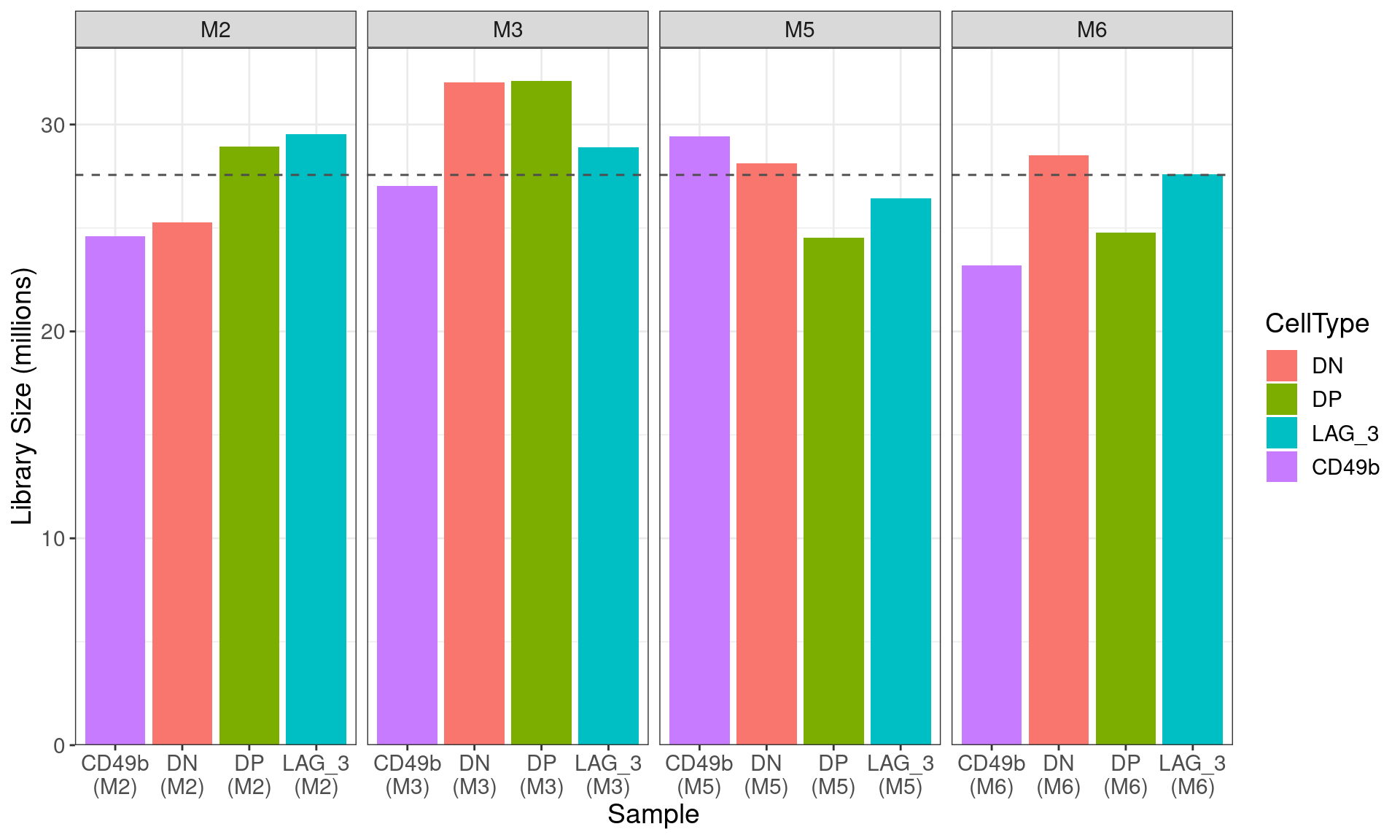

Figure S7a Library sizes for all libraries after summarisation to gene-level counts. The mean library size across all libraries is shown as a dashed horizontal line.

Version	Author	Date
ef7ce0c	Stevie Ped	2023-05-01
8745ba2	Steve Pederson	2022-10-26

Count Densities

dgeFilt %>% 
  cpm(log = TRUE) %>% 
  as_tibble(rownames = "gene_id") %>% 
  pivot_longer(cols = all_of(colnames(dgeFilt)), names_to = "sample", values_to = "logCPM") %>% 
  left_join(dgeFilt$samples, by = "sample") %>% 
  ggplot(aes(logCPM, y = after_stat(density), colour = condition, group = sample)) +
  geom_density() +
  facet_wrap(~mouse) +
  scale_y_continuous(expand = expansion(c(0.01, 0.05)))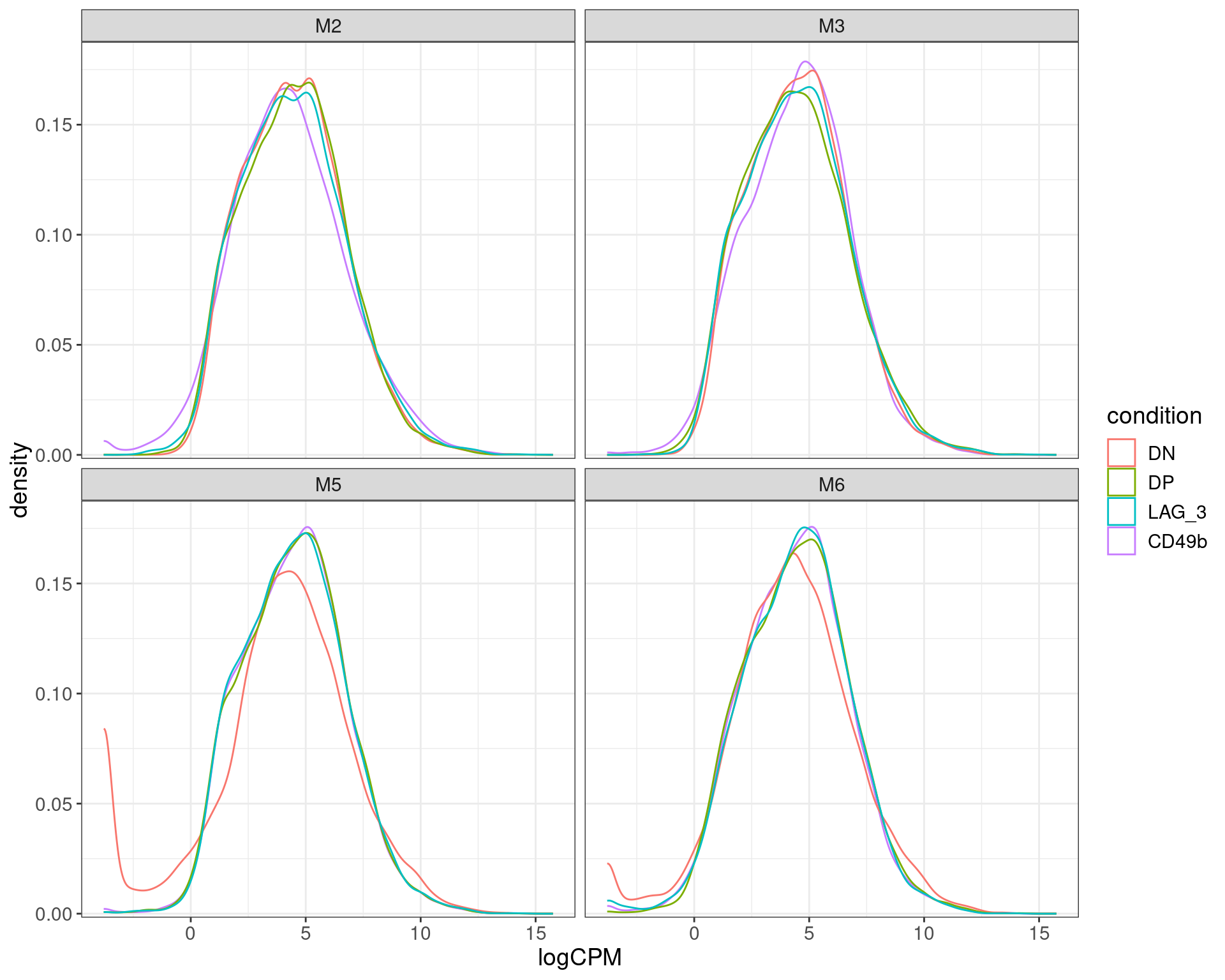

logCPM densisties after removal of undetectable genes. The double negative (DN) samples for both m% and M6 appear to skew to lower overall counts compared to all other samples, with a handful of highly expressed genes likely to dominate the sample.

Version	Author	Date
ef7ce0c	Stevie Ped	2023-05-01
f2ee30e	steveped	2022-11-14
8745ba2	Steve Pederson	2022-10-26

PCA

pca <- dgeFilt %>% 
  cpm(log = TRUE) %>% 
  t() %>% 
  prcomp()
pca %>% 
  broom::tidy() %>% 
  dplyr::rename(sample = row) %>% 
  dplyr::filter(PC %in% c(1, 2)) %>% 
  pivot_wider(names_from = "PC", names_prefix = "PC", values_from = "value") %>% 
  left_join(dgeFilt$samples, by = "sample") %>% 
  ggplot(aes(PC1, PC2, colour = condition)) +
  geom_point(size = 3) +
  geom_text_repel(
    aes(label = label),#str_replace_all(label, " ", "\n")),
    size = 5, max.overlaps = Inf, show.legend = FALSE
  ) +
  labs(
    x = glue("PC1 ({percent(summary(pca)$importance[2, 'PC1'])})"),
    y = glue("PC2 ({percent(summary(pca)$importance[2, 'PC2'])})"),
    colour = "Cell Type"
  )

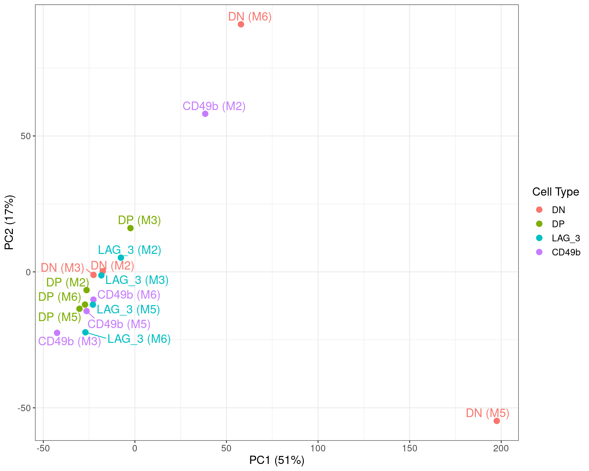
Figure S7b PCA on logCPM values, with the two DN samples identified above clearly showing strong divergence from the remainder of the dataset. The CD49b sample fro M2 also appeared slightly divergent, with the previous density plot also showing a slght skew towards lower overall counts.

Version	Author	Date
ef7ce0c	Stevie Ped	2023-05-01
8745ba2	Steve Pederson	2022-10-26

The above PCA revealed some potential problems with two of the four DN samples. Exclusion of the clear outliers will reduce the number of viable samples within the DN group to 2 and as an alternative, a weighting strategy was instead sought for all samples.

Model Fitting

U <- matrix(1, nrow = ncol(dgeFilt)) %>% 
  set_colnames("Intercept")
v <- voomWithQualityWeights(dgeFilt, design = U)
X <- model.matrix(~0 + condition, data = dgeFilt$samples) %>% 
  set_colnames(str_remove(colnames(.), "condition"))
rho <- duplicateCorrelation(v, X, block=dgeFilt$samples$mouse)$consensus.correlation
v <- voomWithQualityWeights(
  counts = dgeFilt, design = U, block=dgeFilt$samples$mouse, correlation=rho
)
v$design <- X

Sample-level weights were estimated by assuming all samples were drawn from the same group and running voomWithQualityWeights(). After running this, samples were compared within each mouse-of-origin and correlations within mice were estimated using duplicateCorrelation() (\(\rho=\) 0.118). voomWithQualityWeights() was then run again setting mouse as the blocking variable and including the consensus correlations

v$targets %>% 
  ggplot(aes(label, sample.weights, fill = condition)) +
  geom_col() +
  geom_hline(yintercept = 1, linetype = 2, col = "grey30") +
  facet_wrap(~mouse, nrow = 1, scales = "free_x") +
  scale_x_discrete(labels = scales::label_wrap(5)) +
  scale_y_continuous(expand = expansion(c(0, 0.05))) +
  labs(
    x = "Sample", y = "Sample Weights", fill = "Cell Type"
  )

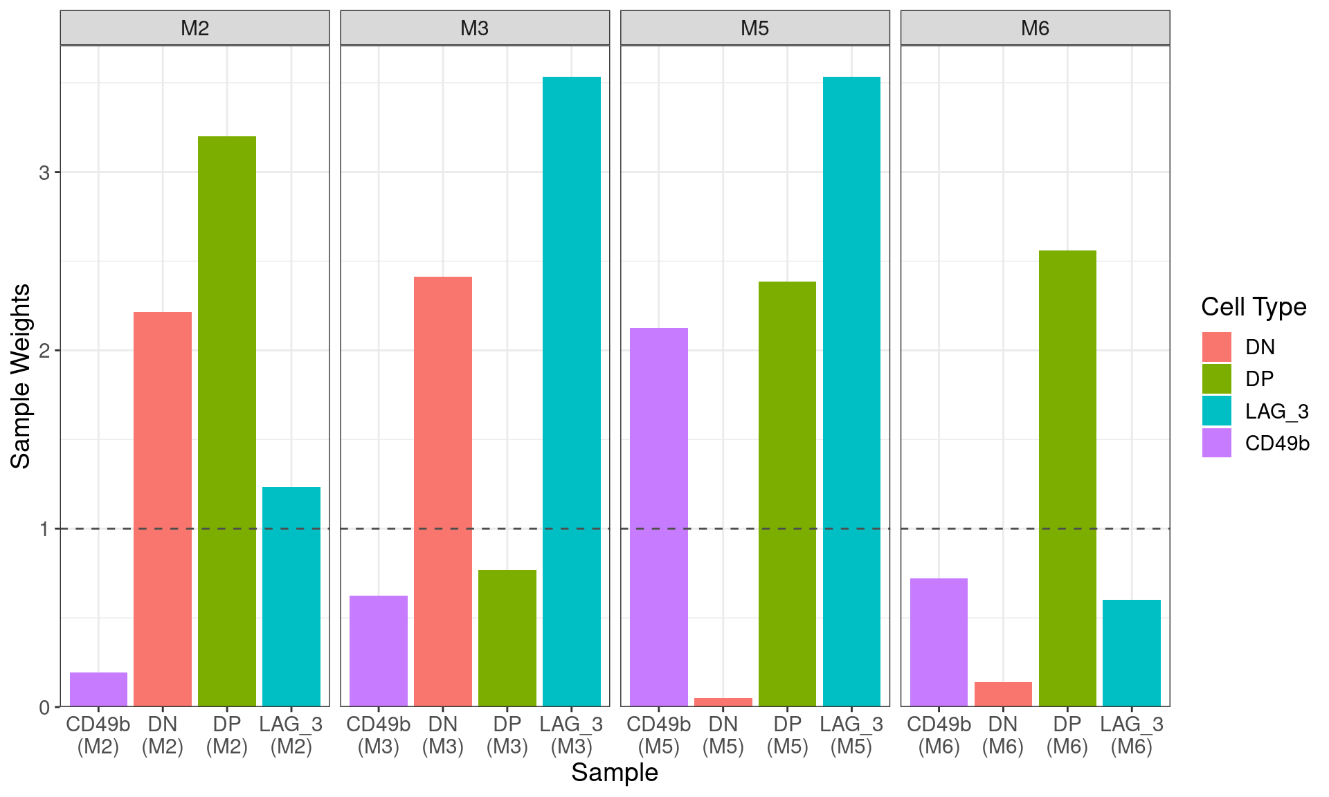
Sample-level weights after running voomWithQualityWeights setting all samples as being drawn from the same condition. The ideal equal wweighting of 1 is shown as the dashed horizontal line, with those samples below this being assumed to be of lower quality than those above the line. Thw two previously identified DN samples were strongly down-weighted, as was the CD49b sample from M2

Version	Author	Date
ef7ce0c	Stevie Ped	2023-05-01
8745ba2	Steve Pederson	2022-10-26

cont.matrix <- makeContrasts(
  DNvLAG3 = DN - LAG_3,
  DNvDP = DN - DP,
  DNvCD49b = DN - CD49b,
  LAG3vCD49b = LAG_3 - CD49b,
  CD49bvDP = CD49b - DP,
  LAG3vDP = LAG_3 - DP,
  levels = X
)
fit <- lmFit(v, design = X, block = v$targets$mouse, correlation = rho) %>% 
  contrasts.fit(cont.matrix) %>%
  # treat()
  eBayes()

Summary Table

top_tables <- colnames(cont.matrix) %>% 
  lapply(function(x) topTable(fit, coef = x, number = Inf)) %>%
  # lapply(function(x) topTreat(fit, coef = x, number = Inf)) %>%
  lapply(as_tibble) %>%
  lapply(mutate, DE = adj.P.Val < 0.05 & abs(logFC) > 1) %>% 
  setNames(colnames(cont.matrix))
top_tables %>% 
  lapply(
    function(x){
      df <- dplyr::filter(x,DE)
      tibble(
        Up = sum(df$logFC > 0),
        Down = sum(df$logFC < 0),
        `Total DE` = Up + Down
      )
    }
  ) %>% 
  bind_rows(.id = "Comparison") %>% 
  pander(
    justify = "lrrr",
    caption = glue(
      "
      Results from each comparison, where genes are considered DE using an FDR
      < 0.05 along with an estimated logFC beyond $\\pm1$. In total, 
      {length(unique(dplyr::filter(bind_rows(top_tables), DE)$gene_id))} 
      unique genes were considered to be DE in at least one comparison.
      "
    )
  )

Results from each comparison, where genes are considered DE using an FDR < 0.05 along with an estimated logFC beyond \(\pm1\). In total, 243 unique genes were considered to be DE in at least one comparison.
Comparison	Up	Down	Total DE
DNvLAG3	46	31	77
DNvDP	27	34	61
DNvCD49b	16	2	18
LAG3vCD49b	111	56	167
CD49bvDP	6	32	38
LAG3vDP	16	17	33

MA Plots

DN Vs. LAG3

top_tables$DNvLAG3 %>% 
  ggplot(aes(AveExpr, logFC)) +
  geom_point(aes(colour = DE), alpha = 0.6) +
  geom_smooth(se = FALSE) +
  geom_label_repel(
    aes(label = gene_name, colour = DE),
    data = . %>% 
      dplyr::filter(DE, logFC > 0) %>% 
      arrange(desc(logFC)) %>% 
      dplyr::slice(1:5),
    size = 5,
    max.overlaps = Inf,
    fontface = "italic",
    show.legend = FALSE
  ) +
  geom_label_repel(
    aes(label = gene_name, colour = DE),
    data = . %>% 
      dplyr::filter(DE, logFC < 0) %>% 
      arrange(logFC) %>% 
      dplyr::slice(1:5),
    size = 5,
    max.overlaps = Inf,
    fontface = "italic",
    show.legend = FALSE
  ) +
  ggtitle("DN Vs. LAG3") +
  scale_colour_manual(values = c("grey30", "red"))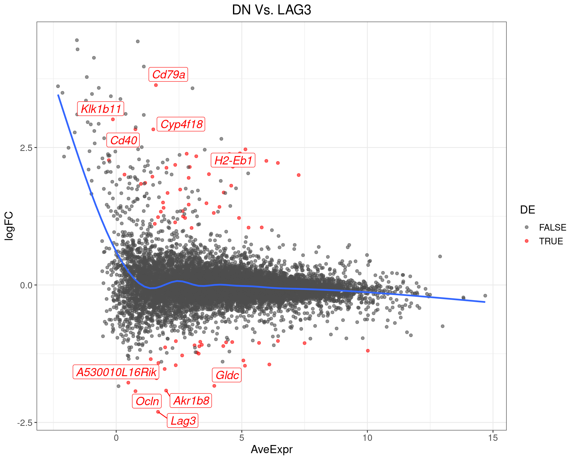

MA-Plot for DN Vs. LAG3. The 5 most up/down-regulated genes are labelled, with the blue line representing a spline through the data.

Version	Author	Date
ef7ce0c	Stevie Ped	2023-05-01
0892674	Steve Pederson	2022-10-26
8745ba2	Steve Pederson	2022-10-26

DN Vs. DP

top_tables$DNvDP %>% 
  ggplot(aes(AveExpr, logFC)) +
  geom_point(aes(colour = DE), alpha = 0.6) +
  geom_smooth(se = FALSE) +
  geom_label_repel(
    aes(label = gene_name, colour = DE),
    data = . %>% 
      dplyr::filter(DE, logFC > 0) %>% 
      arrange(desc(logFC)) %>% 
      dplyr::slice(1:5),
    size = 5,
    max.overlaps = Inf,
    fontface = "italic",
    show.legend = FALSE
  ) +
  geom_label_repel(
    aes(label = gene_name, colour = DE),
    data = . %>% 
      dplyr::filter(DE, logFC < 0) %>% 
      arrange(logFC) %>% 
      dplyr::slice(1:5),
    size = 5,
    max.overlaps = Inf,
    fontface = "italic",
    show.legend = FALSE
  ) +
  ggtitle("DN Vs. DP") +
  scale_colour_manual(values = c("grey30", "red"))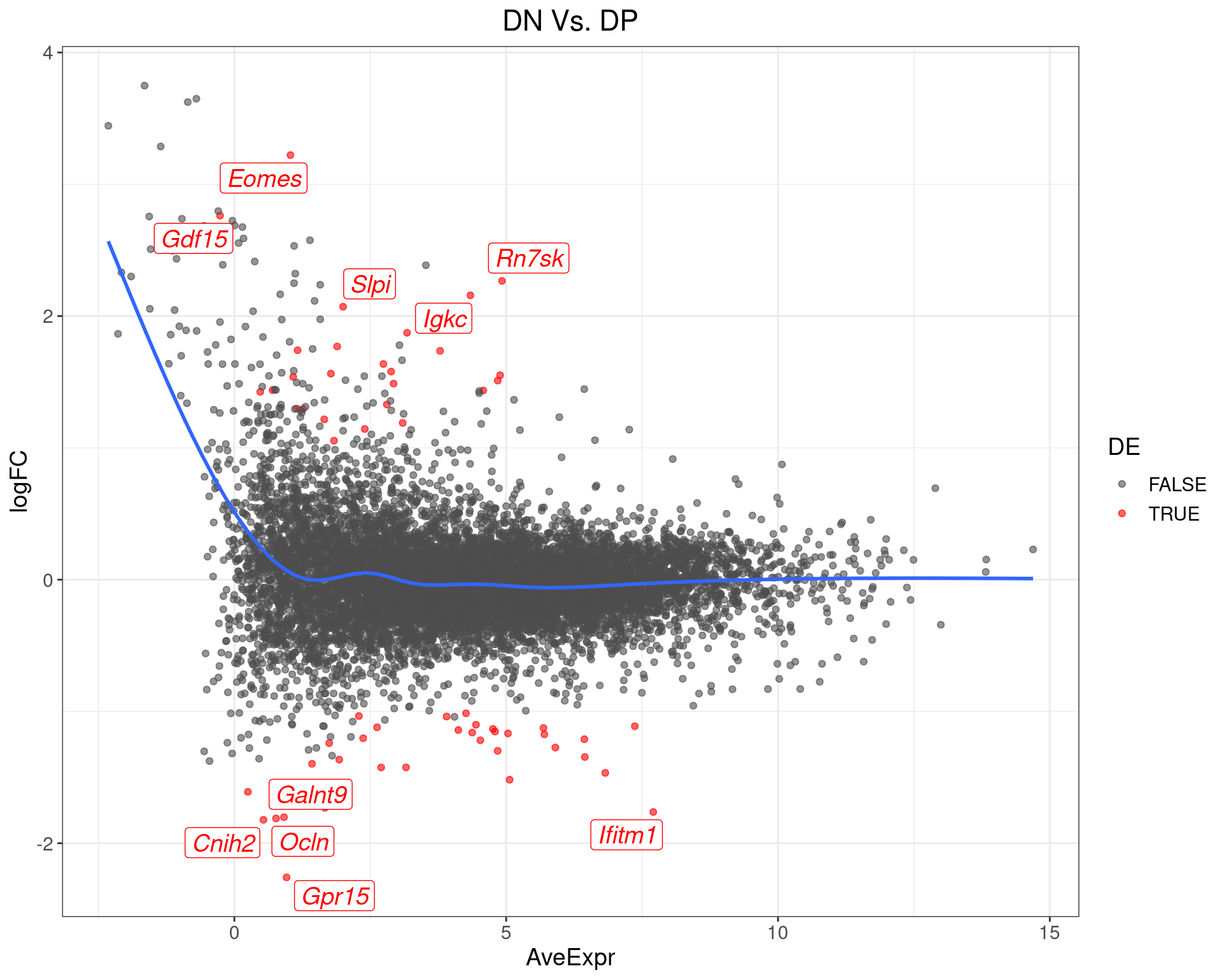

MA-Plot for DN Vs. DP. The 5 most up/down-regulated genes are labelled, with the blue line representing a spline through the data.

Version	Author	Date
ef7ce0c	Stevie Ped	2023-05-01
0892674	Steve Pederson	2022-10-26
8745ba2	Steve Pederson	2022-10-26

DN Vs. CD49b

top_tables$DNvCD49b %>% 
  ggplot(aes(AveExpr, logFC)) +
  geom_point(aes(colour = DE), alpha = 0.6) +
  geom_smooth(se = FALSE) +
  geom_label_repel(
    aes(label = gene_name, colour = DE),
    data = . %>% 
      dplyr::filter(DE, logFC > 0) %>% 
      arrange(desc(logFC)) %>% 
      dplyr::slice(1:5),
    size = 5,
    max.overlaps = Inf,
    fontface = "italic",
    show.legend = FALSE
  ) +
  geom_label_repel(
    aes(label = gene_name, colour = DE),
    data = . %>% 
      dplyr::filter(DE, logFC < 0) %>% 
      arrange(logFC) %>% 
      dplyr::slice(1:5),
    size = 5,
    max.overlaps = Inf,
    fontface = "italic",
    show.legend = FALSE
  ) +
  ggtitle("DN Vs. CD49b") +
  scale_colour_manual(values = c("grey30", "red"))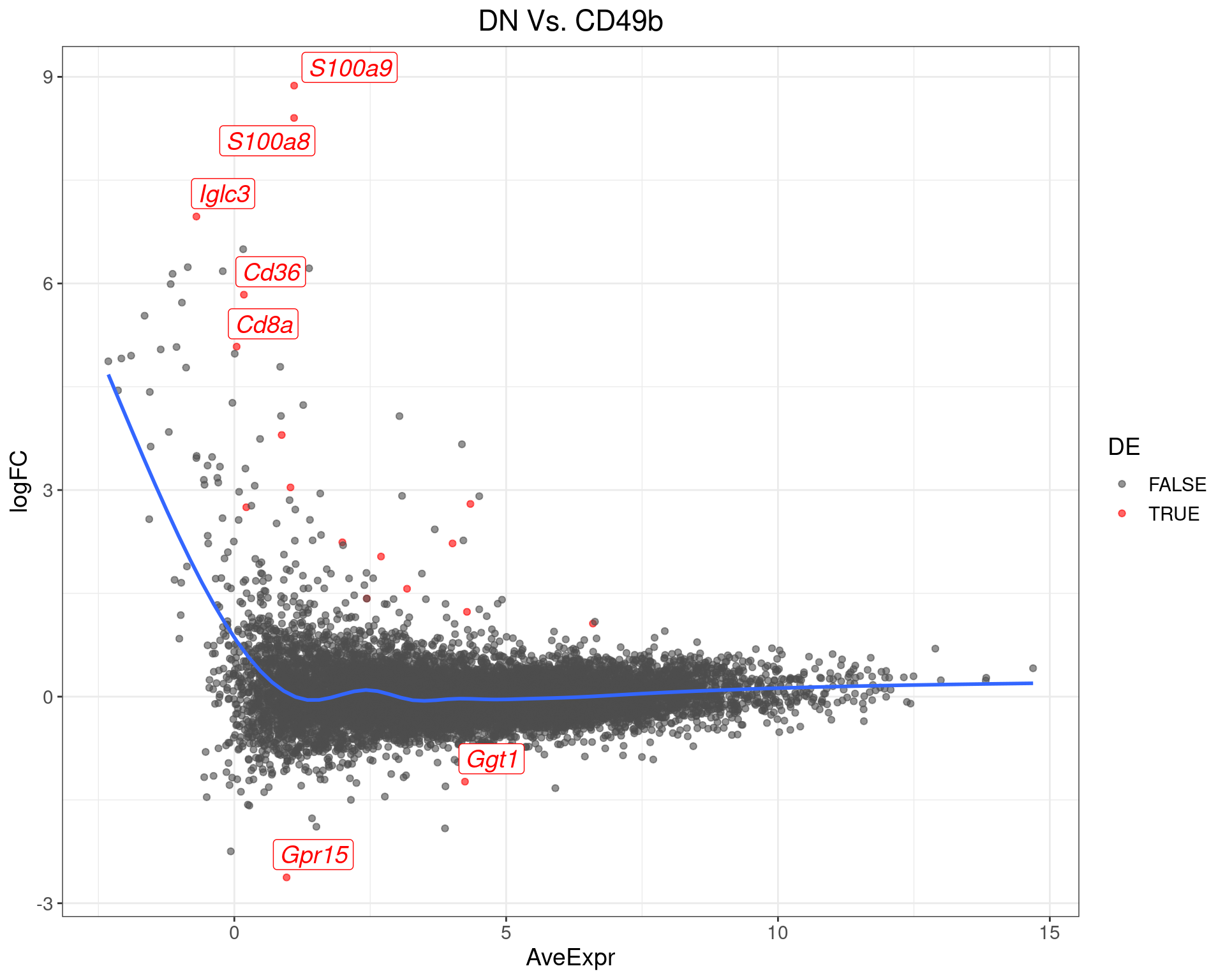

MA-Plot for DN Vs. CD49b The most up/down-regulated genes are labelled, with the blue line representing a spline through the data.

Version	Author	Date
ef7ce0c	Stevie Ped	2023-05-01
0892674	Steve Pederson	2022-10-26
8745ba2	Steve Pederson	2022-10-26

LAG3 Vs. CD49b

top_tables$LAG3vCD49b %>% 
  ggplot(aes(AveExpr, logFC)) +
  geom_point(aes(colour = DE), alpha = 0.6) +
  geom_smooth(se = FALSE) +
  geom_label_repel(
    aes(label = gene_name, colour = DE),
    data = . %>% 
      dplyr::filter(DE, logFC > 0) %>% 
      arrange(desc(logFC)) %>% 
      dplyr::slice(1:5),
    size = 5,
    max.overlaps = Inf,
    fontface = "italic",
    show.legend = FALSE
  ) +
  geom_label_repel(
    aes(label = gene_name, colour = DE),
    data = . %>% 
      dplyr::filter(DE, logFC < 0) %>% 
      arrange(logFC) %>% 
      dplyr::slice(1:5),
    size = 5,
    max.overlaps = Inf,
    fontface = "italic",
    show.legend = FALSE
  ) +
  ggtitle("LAG3 Vs. CD49b") +
  scale_colour_manual(values = c("grey30", "red"))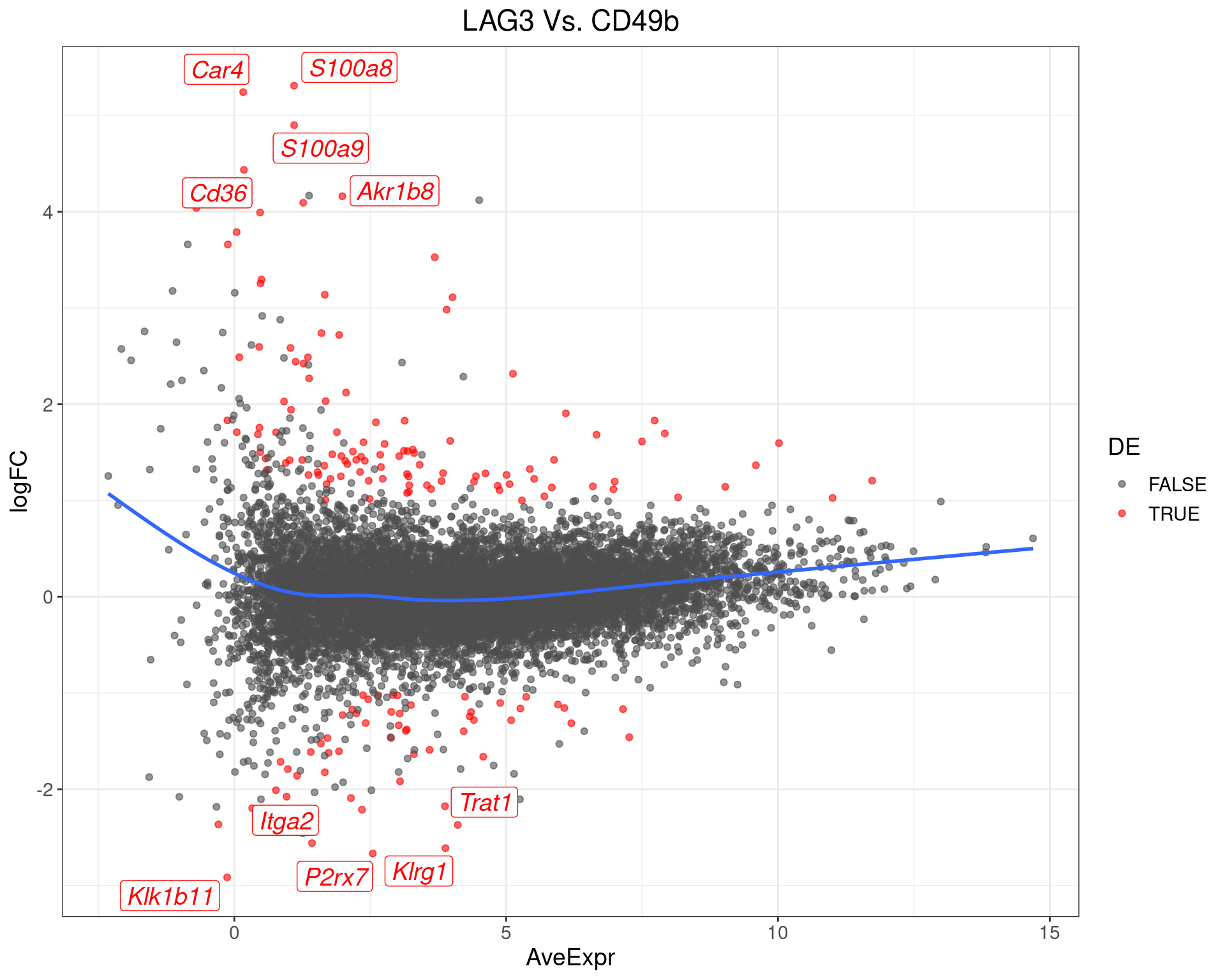

MA-Plot for LAG3 Vs. CD49b. The 5 most up/down-regulated genes are labelled, with the blue line representing a spline through the data.

Version	Author	Date
ef7ce0c	Stevie Ped	2023-05-01
0892674	Steve Pederson	2022-10-26
8745ba2	Steve Pederson	2022-10-26

LAG3 Vs. DP

top_tables$LAG3vDP %>% 
  ggplot(aes(AveExpr, logFC)) +
  geom_point(aes(colour = DE), alpha = 0.6) +
  geom_smooth(se = FALSE) +
  geom_label_repel(
    aes(label = gene_name, colour = DE),
    data = . %>% 
      dplyr::filter(DE, logFC > 0) %>% 
      arrange(desc(logFC)) %>% 
      dplyr::slice(1:5),
    size = 5,
    max.overlaps = Inf,
    fontface = "italic",
    show.legend = FALSE
  ) +
  geom_label_repel(
    aes(label = gene_name, colour = DE),
    data = . %>% 
      dplyr::filter(DE, logFC < 0) %>% 
      arrange(logFC) %>% 
      dplyr::slice(1:5),
    size = 5,
    max.overlaps = Inf,
    fontface = "italic",
    show.legend = FALSE
  ) +
  ggtitle("LAG3 Vs. DP") +
  scale_colour_manual(values = c("grey30", "red"))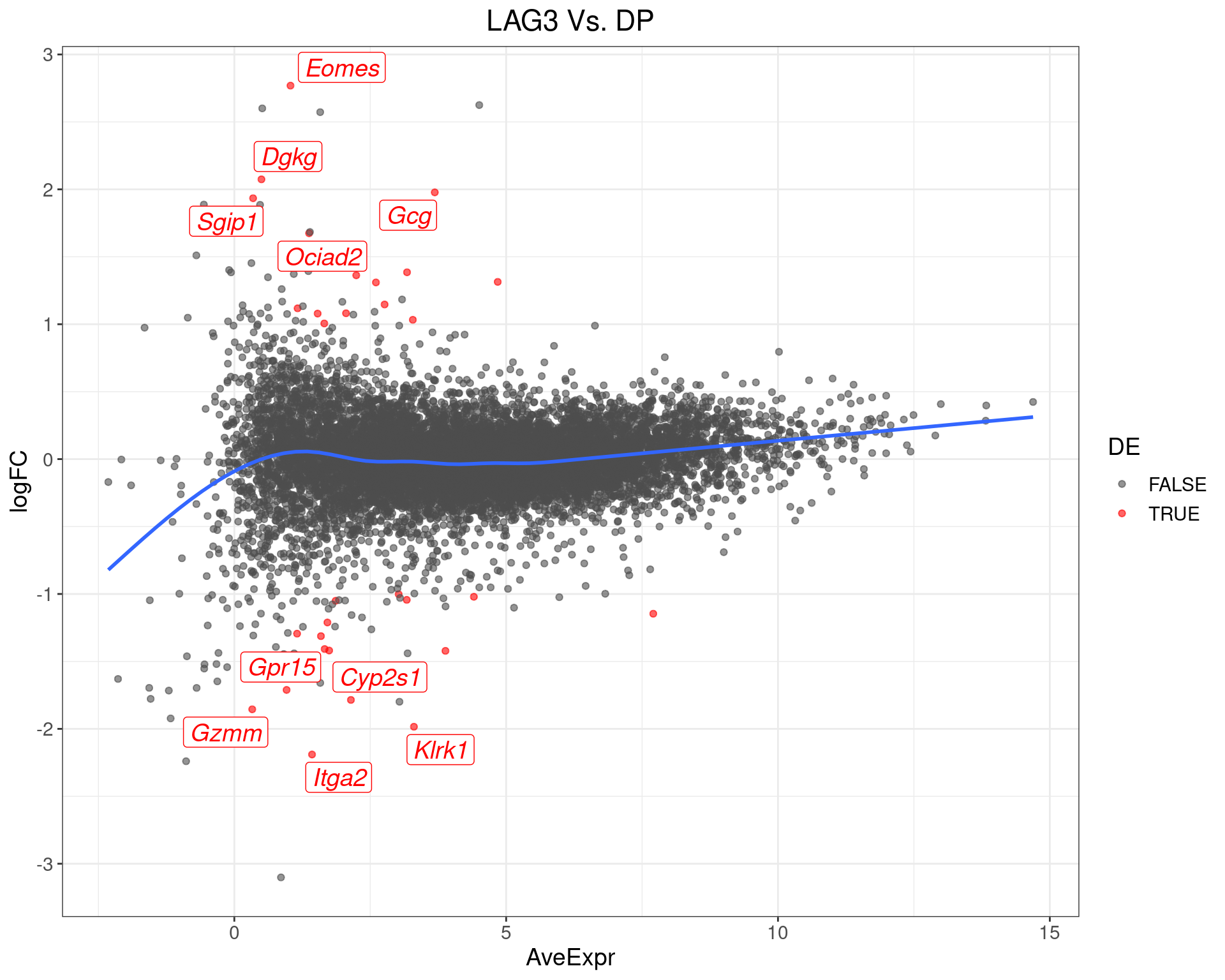

MA-Plot for LAG3 Vs. DP The 5 most up/down-regulated genes are labelled, with the blue line representing a spline through the data.

Version	Author	Date
ef7ce0c	Stevie Ped	2023-05-01
0892674	Steve Pederson	2022-10-26
8745ba2	Steve Pederson	2022-10-26

CD49b Vs. DP

top_tables$CD49bvDP %>% 
  ggplot(aes(AveExpr, logFC)) +
  geom_point(aes(colour = DE), alpha = 0.6) +
  geom_smooth(se = FALSE) +
  geom_label_repel(
    aes(label = gene_name, colour = DE),
    data = . %>% 
      dplyr::filter(DE, logFC > 0) %>% 
      arrange(desc(logFC)) %>% 
      dplyr::slice(1:5),
    size = 5,
    max.overlaps = Inf,
    fontface = "italic",
    show.legend = FALSE
  ) +
  geom_label_repel(
    aes(label = gene_name, colour = DE),
    data = . %>% 
      dplyr::filter(DE, logFC < 0) %>% 
      arrange(logFC) %>% 
      dplyr::slice(1:5),
    size = 5,
    max.overlaps = Inf,
    fontface = "italic",
    show.legend = FALSE
  ) +
  ggtitle("CD49b Vs. DP") +
  scale_colour_manual(values = c("grey30", "red"))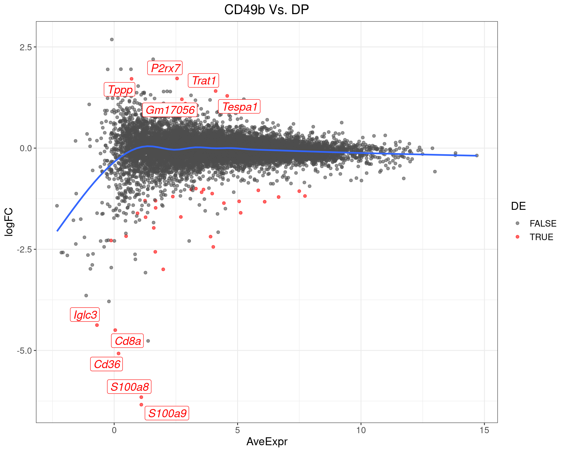

MA-Plot for CD49b Vs. DP. The 5 most up/down-regulated genes are labelled, with the blue line representing a spline through the data.

Version	Author	Date
ef7ce0c	Stevie Ped	2023-05-01
0892674	Steve Pederson	2022-10-26
8745ba2	Steve Pederson	2022-10-26

Volcano Plots

DN Vs. LAG3

top_tables$DNvLAG3 %>% 
  ggplot(aes(logFC, -log10(P.Value))) +
  geom_point(aes(colour = DE), alpha = 0.6) +
  geom_label_repel(
    aes(label = gene_name, colour = DE),
    data = . %>% 
      dplyr::filter(DE) %>% 
      arrange(P.Value) %>% 
      dplyr::slice(1:20),
    size = 5,
    max.overlaps = Inf,
    fontface = "italic",
    show.legend = FALSE
  ) +
  ggtitle("DN Vs. LAG3") +
  scale_colour_manual(values = c("grey30", "red")) +
  theme(text = element_text(size = 16))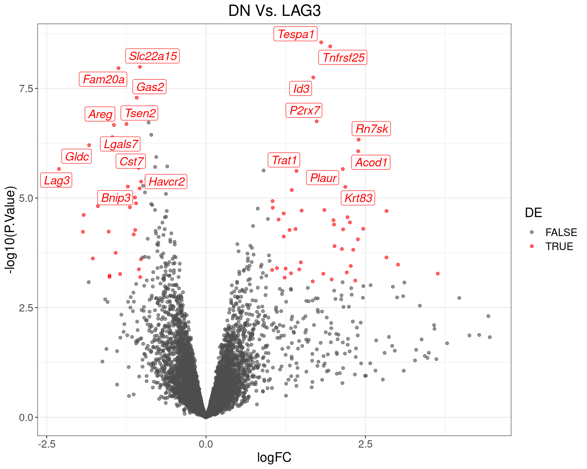

Volcano Plot for DN Vs. LAG3. The (up to) 20 most highly-ranked genes are labelled.

Version	Author	Date
ef7ce0c	Stevie Ped	2023-05-01
ee4bb47	steveped	2022-11-17
0892674	Steve Pederson	2022-10-26
8745ba2	Steve Pederson	2022-10-26

DN Vs. DP

top_tables$DNvDP %>% 
  ggplot(aes(logFC, -log10(P.Value))) +
  geom_point(aes(colour = DE), alpha = 0.6) +
  geom_label_repel(
    aes(label = gene_name, colour = DE),
    data = . %>% 
      dplyr::filter(DE) %>% 
      arrange(P.Value) %>% 
      dplyr::slice(1:20),
    size = 5,
    max.overlaps = Inf,
    fontface = "italic",
    show.legend = FALSE
  ) +
  ggtitle("DN Vs. DP") +
  scale_colour_manual(values = c("grey30", "red")) +
  theme(text = element_text(size = 16))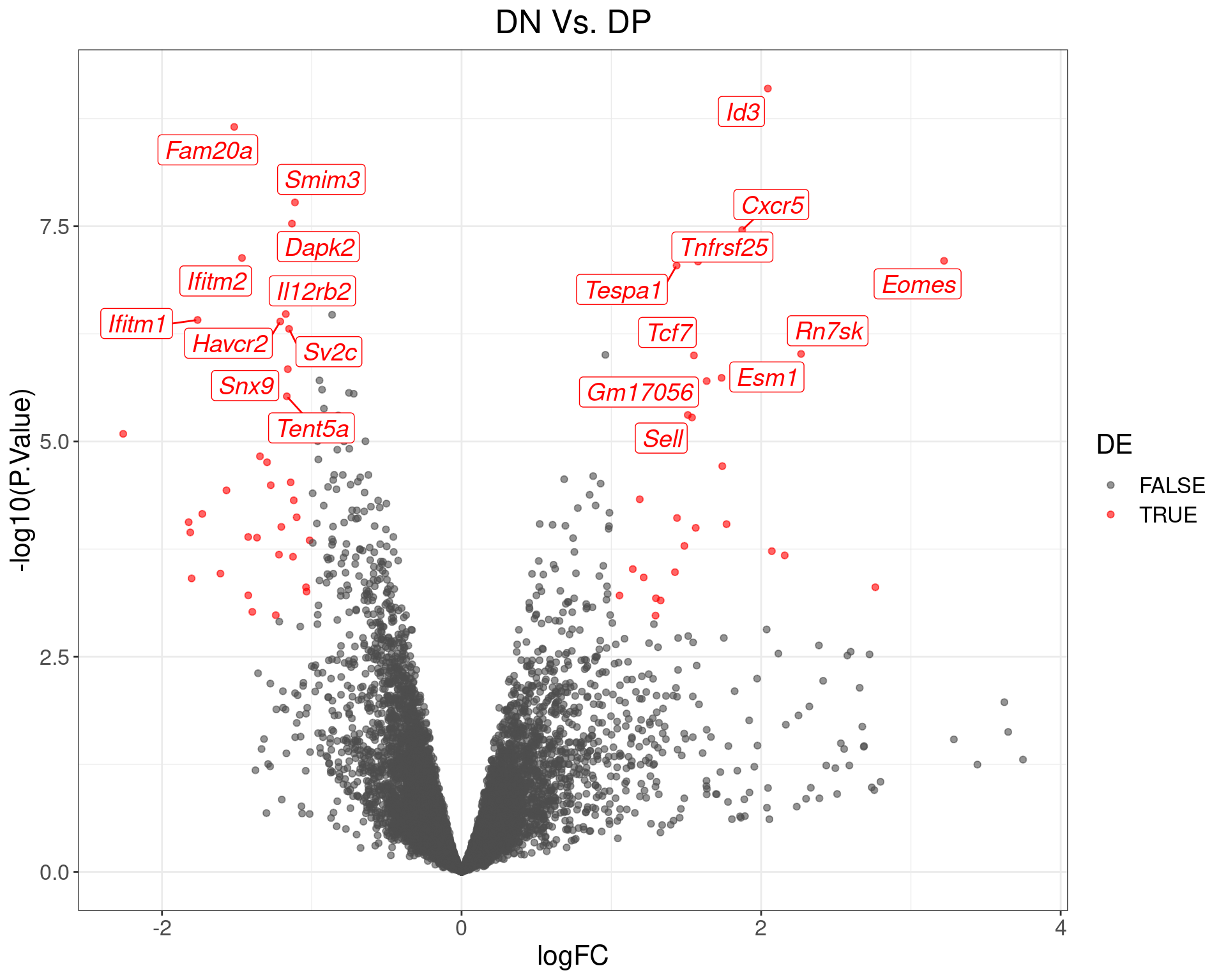

Volcano Plot for DN Vs. DP. The (up to) 20 most highly-ranked genes are labelled.

Version	Author	Date
ef7ce0c	Stevie Ped	2023-05-01
ee4bb47	steveped	2022-11-17
0892674	Steve Pederson	2022-10-26
8745ba2	Steve Pederson	2022-10-26

DN Vs. CD49b

top_tables$DNvCD49b %>% 
  ggplot(aes(logFC, -log10(P.Value))) +
  geom_point(aes(colour = DE), alpha = 0.6) +
  geom_label_repel(
    aes(label = gene_name, colour = DE),
    data = . %>% 
      dplyr::filter(DE) %>% 
      arrange(P.Value) %>% 
      dplyr::slice(1:20),
    size = 5,
    max.overlaps = Inf,
    fontface = "italic",
    show.legend = FALSE
  ) +
  ggtitle("DN Vs. CD49b") +
  scale_colour_manual(values = c("grey30", "red")) +
  theme(text = element_text(size = 16))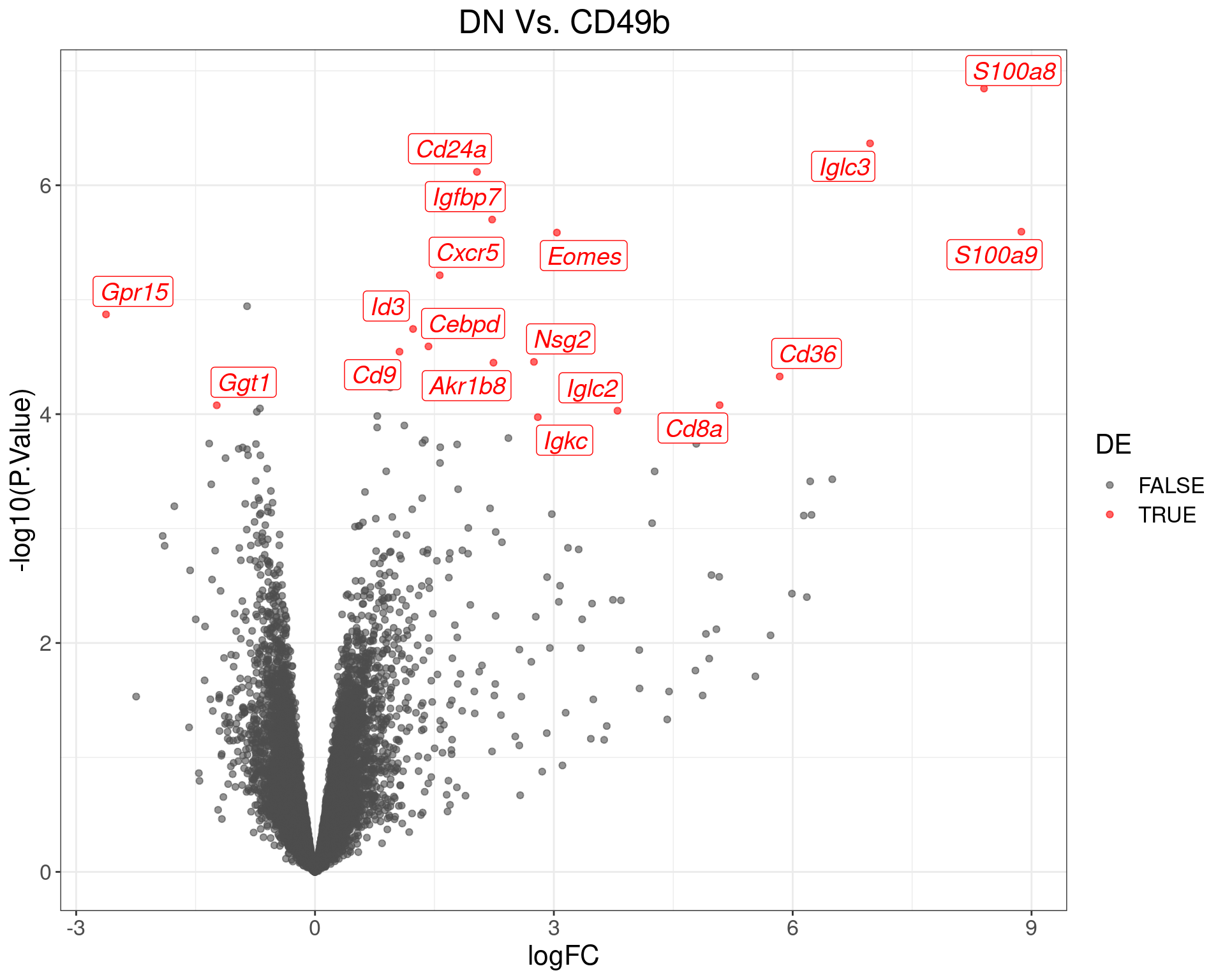

Volcano Plot for DN Vs. CD49b. The (up to) 20 most highly-ranked genes are labelled.

Version	Author	Date
ef7ce0c	Stevie Ped	2023-05-01
ee4bb47	steveped	2022-11-17
0892674	Steve Pederson	2022-10-26
8745ba2	Steve Pederson	2022-10-26

LAG3 Vs. CD49b

top_tables$LAG3vCD49b %>% 
  ggplot(aes(logFC, -log10(P.Value))) +
  geom_point(aes(colour = DE), alpha = 0.6) +
  geom_label_repel(
    aes(label = gene_name, colour = DE),
    data = . %>% 
      dplyr::filter(DE) %>% 
      arrange(P.Value) %>% 
      dplyr::slice(1:20),
    size = 5,
    max.overlaps = Inf,
    fontface = "italic",
    show.legend = FALSE
  ) +
  ggtitle("LAG3 Vs. CD49b") +
  scale_colour_manual(values = c("grey30", "red")) +
  theme(text = element_text(size = 16))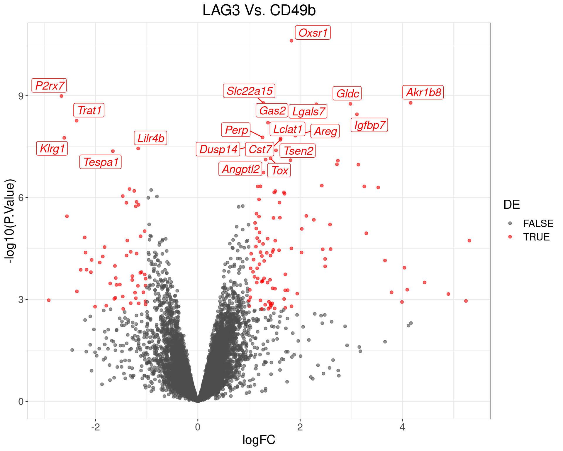

Volcano Plot for LAG3 Vs. CD49b. The (up to) 20 most highly-ranked genes are labelled.

Version	Author	Date
ef7ce0c	Stevie Ped	2023-05-01
ee4bb47	steveped	2022-11-17
0892674	Steve Pederson	2022-10-26
8745ba2	Steve Pederson	2022-10-26

LAG3 Vs. DP

top_tables$LAG3vDP %>% 
  ggplot(aes(logFC, -log10(P.Value))) +
  geom_point(aes(colour = DE), alpha = 0.6) +
  geom_label_repel(
    aes(label = gene_name, colour = DE),
    data = . %>% 
      dplyr::filter(DE) %>% 
      arrange(P.Value) %>% 
      dplyr::slice(1:20),
    size = 5,
    max.overlaps = Inf,
    fontface = "italic",
    show.legend = FALSE
  ) +
  ggtitle("LAG3 Vs. DP") +
  scale_colour_manual(values = c("grey30", "red")) +
  theme(text = element_text(size = 16))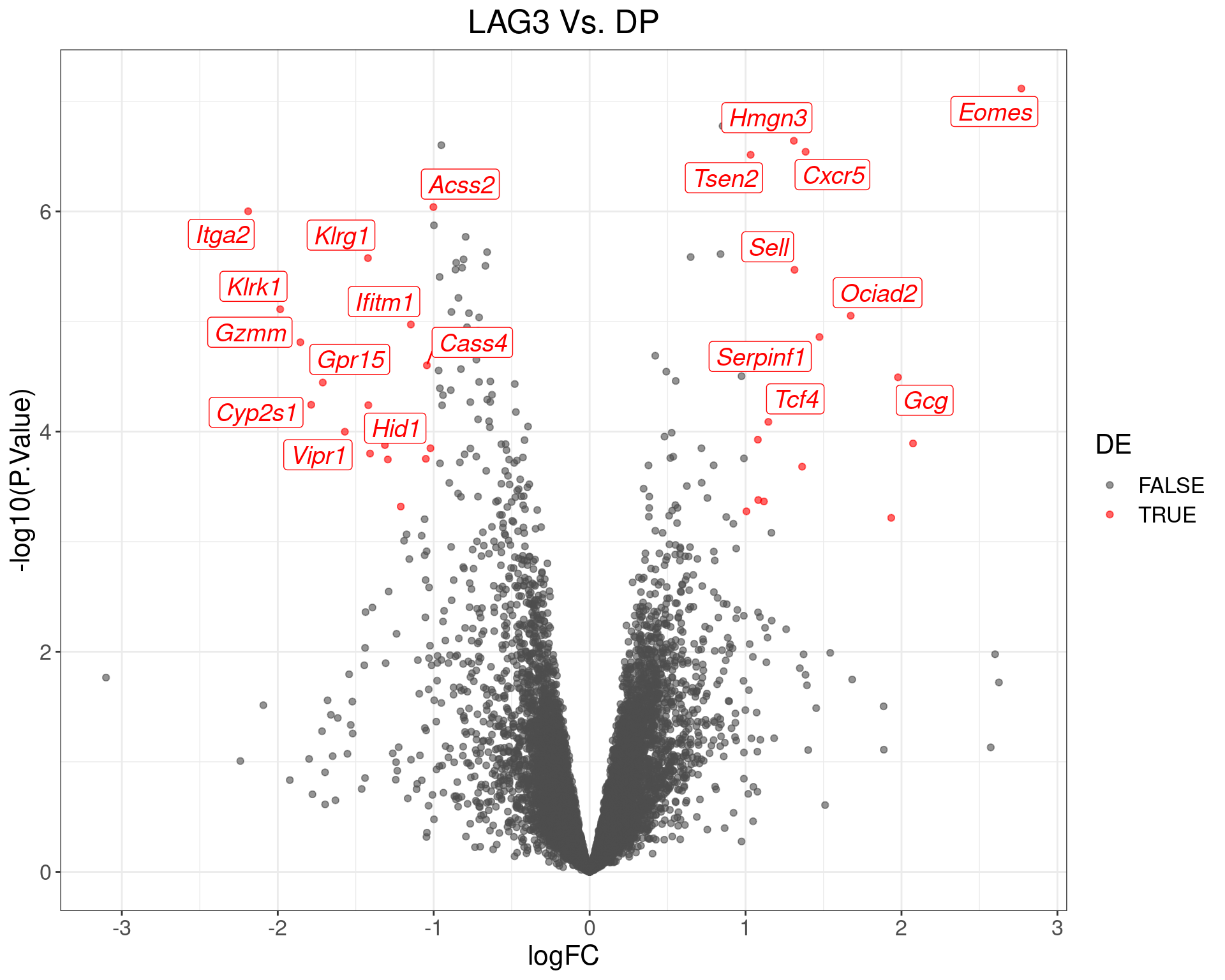

Volcano Plot for LAG3 Vs. DP. The (up to) 20 most highly-ranked genes are labelled.

Version	Author	Date
ef7ce0c	Stevie Ped	2023-05-01
ee4bb47	steveped	2022-11-17
0892674	Steve Pederson	2022-10-26
8745ba2	Steve Pederson	2022-10-26

CD49b Vs. DP

top_tables$CD49bvDP %>% 
  ggplot(aes(logFC, -log10(P.Value))) +
  geom_point(aes(colour = DE), alpha = 0.6) +
  geom_label_repel(
    aes(label = gene_name, colour = DE),
    data = . %>% 
      dplyr::filter(DE) %>% 
      arrange(P.Value) %>% 
      dplyr::slice(1:20),
    size = 5,
    max.overlaps = Inf,
    fontface = "italic",
    show.legend = FALSE
  ) +
  ggtitle("CD49b Vs. DP") +
  scale_colour_manual(values = c("grey30", "red")) +
  theme(text = element_text(size = 16))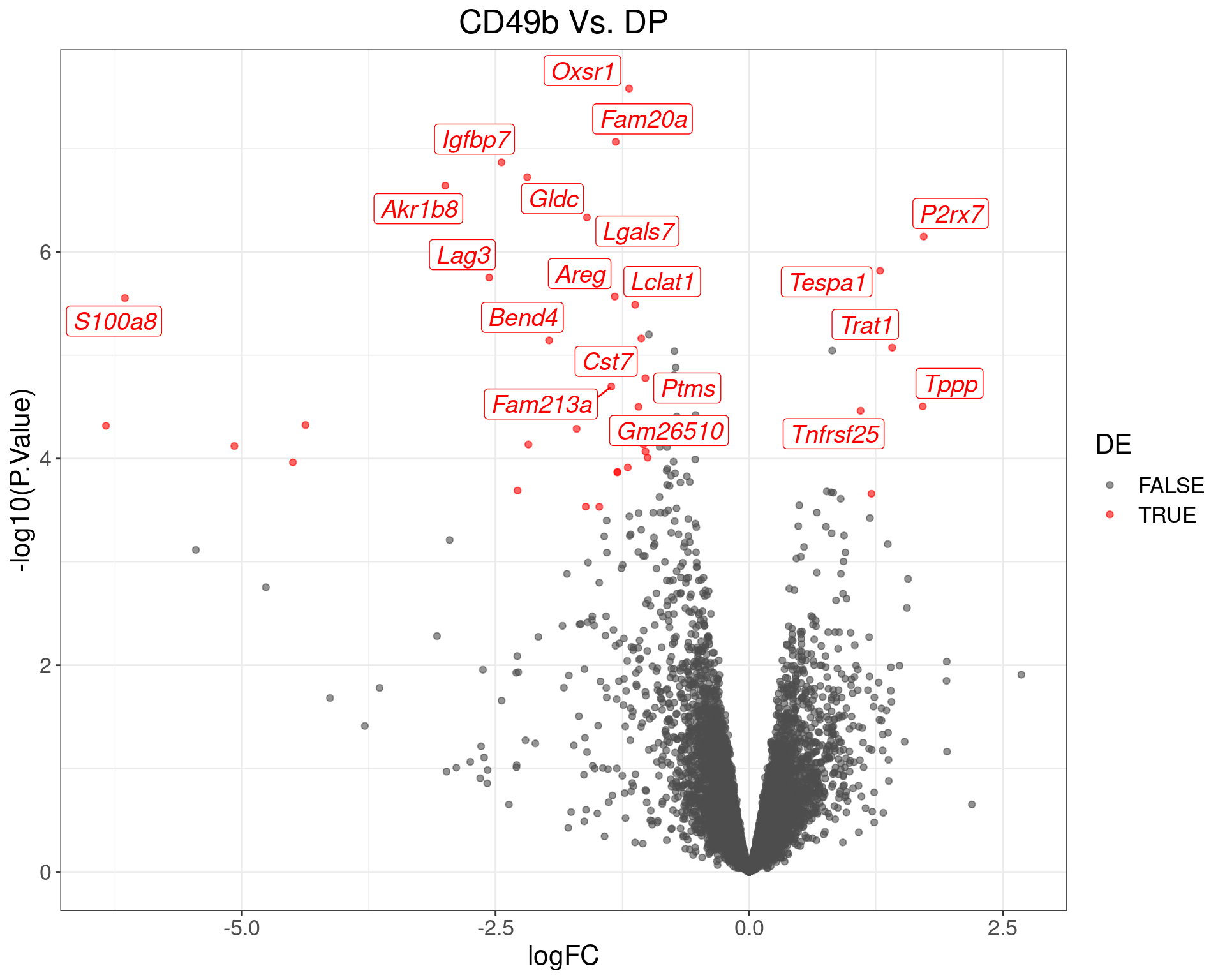

Volcano Plot for CD49b Vs. DP. The (up to) 20 most highly-ranked genes are labelled.

Version	Author	Date
ef7ce0c	Stevie Ped	2023-05-01
ee4bb47	steveped	2022-11-17
0892674	Steve Pederson	2022-10-26
8745ba2	Steve Pederson	2022-10-26

DE Gene Summary

UpSet Plot

all_de <- top_tables %>% 
  lapply(dplyr::filter, DE) %>%
  bind_rows() %>% 
  pull("gene_id") %>% 
  unique()
top_tables %>% 
  lapply(dplyr::filter, adj.P.Val < 0.05, gene_id %in% all_de) %>%
  lapply(dplyr::select, gene_id) %>% 
  bind_rows(.id = "comparison") %>% 
  mutate(DE = TRUE, comparison = str_replace_all(comparison, "v", " Vs. ")) %>% 
  pivot_wider(names_from = comparison, values_from = DE, values_fill = FALSE) %>% 
  upset(
    intersect = str_replace_all(names(top_tables), "v", " Vs. "),
    base_annotations = list(
      'Intersection size' = intersection_size(
        bar_number_threshold = 1, width = 0.9, text = list(size = 5)
      ) +
        scale_y_continuous(expand = expansion(c(0, 0.1))) +
        scale_fill_manual(values = c(bars_color = "grey20")) +
        theme(
          panel.grid = element_blank(), 
          axis.title = element_text(size = 14),
          axis.text = element_text(size = 14)
        )
    ),
    sort_sets = FALSE,
    set_sizes = upset_set_size() +
      geom_text(
        aes(label = comma(after_stat(count))), 
        stat = 'count', hjust = 1.1, size = 5
      ) +
      scale_y_reverse(expand = expansion(c(0.25, 0))) +
      theme(
        panel.grid = element_blank(), axis.text = element_text(size = 14),
        axis.title = element_text(size = 14)
      ),
    queries = list(
      upset_query(
        intersect = str_subset(colnames(.), "LAG3"),
        fill = "red", color = "red",
        only_components = c("intersections_matrix", "Intersection size")
      ),
      upset_query(
        intersect = str_subset(colnames(.), "CD49"),
        fill = "forestgreen", color = "forestgreen",
        only_components = c("intersections_matrix", "Intersection size")
      ),
      upset_query(
        intersect = str_subset(colnames(.), "DN"),
        fill = "blue", color = "blue",
        only_components = c("intersections_matrix", "Intersection size")
      )
    ),
    min_size = 2
  ) +
  labs(x = "Group") +
  theme(
    panel.grid = element_blank(), axis.text = element_text(size = 14),
    axis.title = element_text(size = 14)
  )

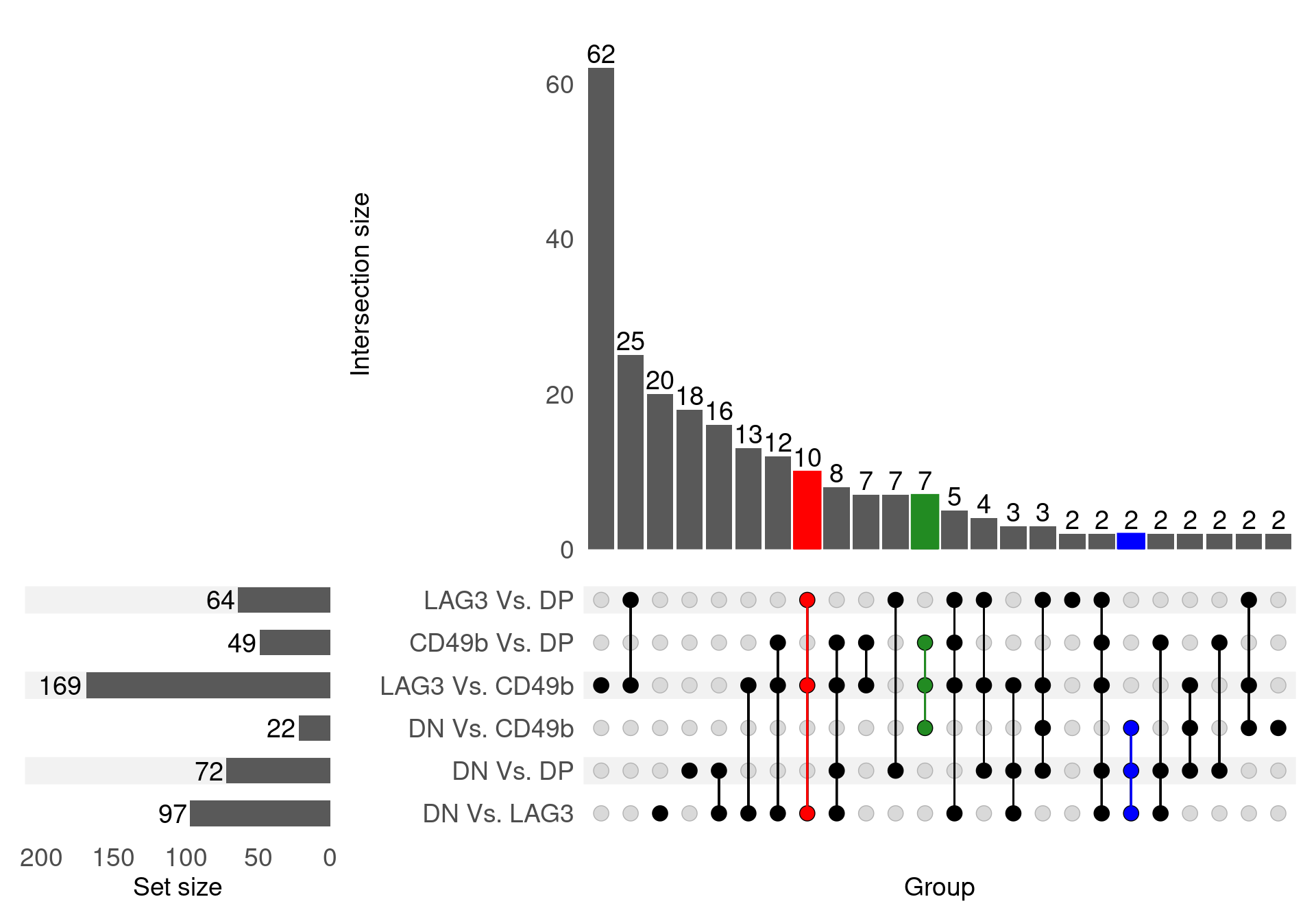
UpSet plot for all DE genes. A complete list of DE genes was obtained by finding all genes considered DE after filtering by FDR and logFC across all comparisons. For the purposes of comparison, any genes in this complete list were considered as DE in a comparison if receiving an FDR-adjusted p-value < 0.05 in order for this figure to give a more accurate picture across all 6 comparisons, and avoiding any misleading results from the use of a hard cutoff. The genes DE in all LAG3 comparisons are highlighted in red, whilst the CD49b signature is shown in green and the DN signature is shown in blue. No clear DP signature was evident in this viewpoint.

Version	Author	Date
ef7ce0c	Stevie Ped	2023-05-01
63a6ba6	steveped	2022-11-24

Heatmaps

In order to visualise the data using heatmaps, the average expression within each cell type was calculated.

grp_coef <- dgeList %>%
  cpm(log = TRUE) %>% 
  as_tibble(rownames = "gene_id") %>% 
  pivot_longer(
    cols = all_of(colnames(v)), names_to = "sample", values_to = "logCPM"
  ) %>% 
  left_join(v$targets) %>% 
  group_by(gene_id, condition) %>% 
  # summarise(logCPM = weighted.mean(logCPM, sample.weights)) %>%
  summarise(logCPM = mean(logCPM)) %>%
  pivot_wider(names_from = "condition", values_from = "logCPM") %>% 
  as.data.frame() %>%
  column_to_rownames("gene_id") %>% 
  as.matrix()

Key Signatures

signatures <- top_tables %>% 
  bind_rows(.id = "comparison") %>% 
  dplyr::filter(gene_id %in% all_de, adj.P.Val < 0.05) %>% 
  dplyr::select(comparison, gene_id, gene_name, AveExpr) %>% 
  chop(comparison) %>% 
  dplyr::filter(vapply(comparison, length, integer(1)) == 3) %>% 
  dplyr::mutate(
    Signature = case_when(
      vapply(comparison, function(x) sum(str_detect(x, "CD49")) == 3, logical(1)) ~ "Cd49b+",
      vapply(comparison, function(x) sum(str_detect(x, "LAG3")) == 3, logical(1)) ~ "Lag3+",
      vapply(comparison, function(x) sum(str_detect(x, "DN")) == 3, logical(1)) ~ "DN",
      TRUE ~ "Other"
    )
  ) %>% 
  dplyr::filter(Signature != "Other") %>% 
  dplyr::select(starts_with("gene"), Signature, AveExpr) %>% 
  arrange(Signature, desc(AveExpr)) %>% 
  as.data.frame() %>% 
  column_to_rownames("gene_id")
sig_heat <- grp_coef[rownames(signatures),] %>% 
  pheatmap(
    annotation_row = dplyr::select(signatures, Signature),
    cluster_rows = FALSE, cluster_cols = FALSE,
    labels_row = setNames(signatures$gene_name, rownames(signatures)),
    labels_col = c(DN = "DN", DP = "DP", LAG_3 = "Lag3+", CD49b = "CD49b+"),
    gaps_row = cumsum(c(
      sum(signatures$Signature == "Cd49b+"),
      sum(signatures$Signature == "DN")
    )),
    color = hcl.colors(101, "inferno"),
    cutree_rows = 7,
    cellwidth = 25,
    cellheight = 15,
    annotation_colors = list(
      Signature = c("Cd49b+" = "forestgreen", "DN" = "blue", "Lag3+" = "red")
    ), fontsize = 12,
    silent = TRUE
  ) %>% 
  .[["gtable"]]
sig_heat$grobs[[3]]$gp <- gpar(fonsize = 12, fontface = "italic")
png(
  here::here("docs", "assets", "sig_heat.png"),
  height = 6, width = 4, units = "in", res = 300
)
grid.newpage()
grid.draw(sig_heat)
dev.off()
pdf(
  here::here("docs", "assets", "sig_heat.pdf"),
  height = 6, width = 4
)
grid.newpage()
grid.draw(sig_heat)
dev.off()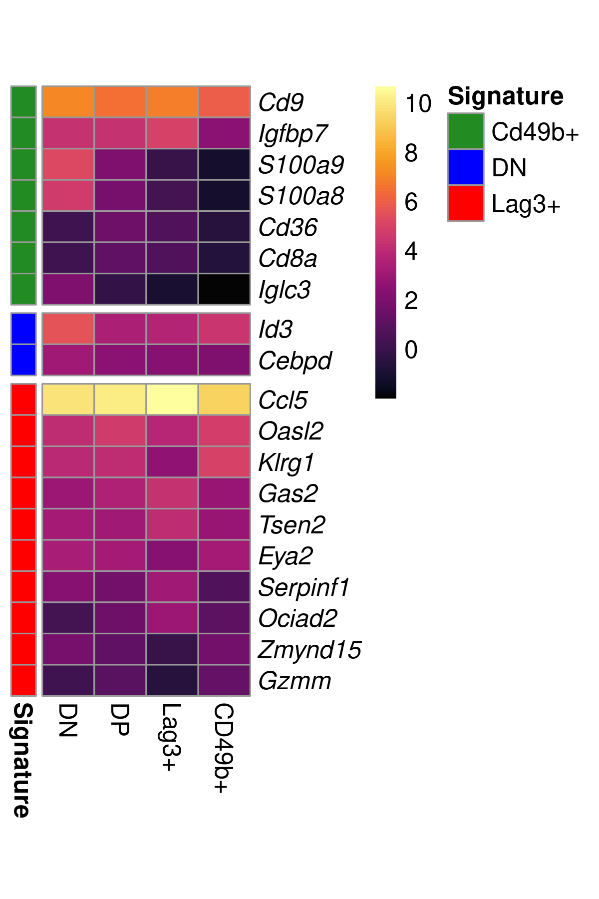

Expression values from genes in each of the key signatures defined in the previous UpSet plot were plotted. Within each signature genes are arranged in order of average expression. Most genes in the CD49b+ signature showed lower expression in this cell type, whilst patterns were more varied for each of the other signatures. The pdf of this image is available here

High Confidence Genes

highConf_df <- tribble(
  ~Group, ~gene_name,
  "Treg", "Foxp3",
  "Treg", "Ikzf4",
  "Treg", "Il1rl1",
  "Treg", "Il2ra",
  "Treg", "Il2rb",
  "Th2", "Gata3",
  "Th2", "Il4",
  "Th2", "Il5",
  "Th2", "Il13",
  "Th17", "Rorc",
  "Th17", "Il17a",
  "Th17", "Il17f",
  "Th17", "Ccr6",
  "Th1", "Tnf",
  "Th1", "Tbx21",
  "Th1", "Cxcr3",
  "Th1", "Cxcr6",
  "Th1", "Ifng",
  "Tfh", "Bcl6",
  "Tfh", "Cxcr5",
  "Tfh", "Tcf7",
  "Tfh", "Tox2",
  "Tr1", "Lag3",
  "Tr1", "Itga2",
  "Tr1", "Eomes",
  "Tr1", "Tgfb1",
  "Tr1", "Il21",
  "Tr1", "Ccr5",
  "Tr1", "Il10",
  "Tr1", "Pdcd1",
  "Tr1", "Tigit",
  "Tr1", "Maf",
  "Tr1", "Batf",
  "Tr1", "Irf1",
  "Tr1", "Stat1",
  "Tr1", "Stat3",
  "Tr1", "Gzmb",
  "Tr1", "Icos",
  "Tr1", "Ctla4",
  "Tr1", "Havcr2",
  "Tr1", "Cd226",
  "Tr1", "Prdm1",
  "Tr1", "Ahr",
  "Tr1", "Irf4",
) %>%
  left_join(
    # dplyr::select(dgeFilt$genes, gene_name, gene_id)
    dplyr::select(dgeList$genes, gene_name, gene_id)
  ) %>% 
  as.data.frame() %>% 
  column_to_rownames("gene_id")
p <- grp_coef[rownames(highConf_df),] %>% 
  pheatmap(
    # cluster_rows = FALSE,
    cluster_cols = FALSE,
    clustering_method = "complete",
    labels_row = setNames(highConf_df$gene_name, rownames(highConf_df)),
    labels_col = c(DN = "DN", DP = "DP", LAG_3 = "Lag3+", CD49b = "CD49b+"),
    color = hcl.colors(101, "inferno"),
    cellwidth = 15, fontsize = 13,
    cutree_rows = 4,
    # annotation_row = dplyr::select(highConf_df, Group),
    # annotation_colors = list(
    #   Group = setNames(RColorBrewer::brewer.pal(6, "Accent"), unique(highConf_df$Group))
    # ),
    silent = TRUE
  ) %>% 
  .[["gtable"]]
p$grobs[[4]]$gp <- gpar(fontsize = 13, fontface = "italic")
bu <- 0.07
grp_df <- highConf_df %>%
  mutate(i = seq_along(gene_name) / nrow(.)) %>% 
  group_by(Group) %>% 
  summarise(
    y_max = 1 - min(i) + 0.004,
    y_min = 1 - max(i) - 0.003
  ) %>% 
  mutate(
    y_max = bu + (1 - bu) * y_max,
    y_min = bu + (1 - bu) * y_min
  ) %>% 
  split(.$Group)
png(
  here::here("docs", "assets", "highconf_heat.png"),
  width = 5, height = 11, res = 300, units = "in"
)
grid.newpage()
grid.draw(p)
# grp_df %>% 
#   lapply(
#     function(x) {
#       grid.lines(
#         x = 0.295, 
#         y = c(x$y_max, x$y_min), 
#         gp = gpar(lwd = 2.5)
#       )
#       grid.text(
#         x$Group, x = 0.25,
#         y = 0.5 * (x$y_min + x$y_max) + 0.01
#       )
#     }
#   )
dev.off()
pdf(
  here::here("docs", "assets", "highconf_heat.pdf"),
  width = 5, height = 11
)
grid.newpage()
grid.draw(p)
# grp_df %>%
#   lapply(
#     function(x) {
#       grid.lines(
#         x = 0.295,
#         y = c(x$y_max, x$y_min),
#         gp = gpar(lwd = 2.5)
#       )
#       grid.text(
#         x$Group, x = 0.25,
#         y = 0.5 * (x$y_min + x$y_max) + 0.01
#       )
#     }
#   )
dev.off()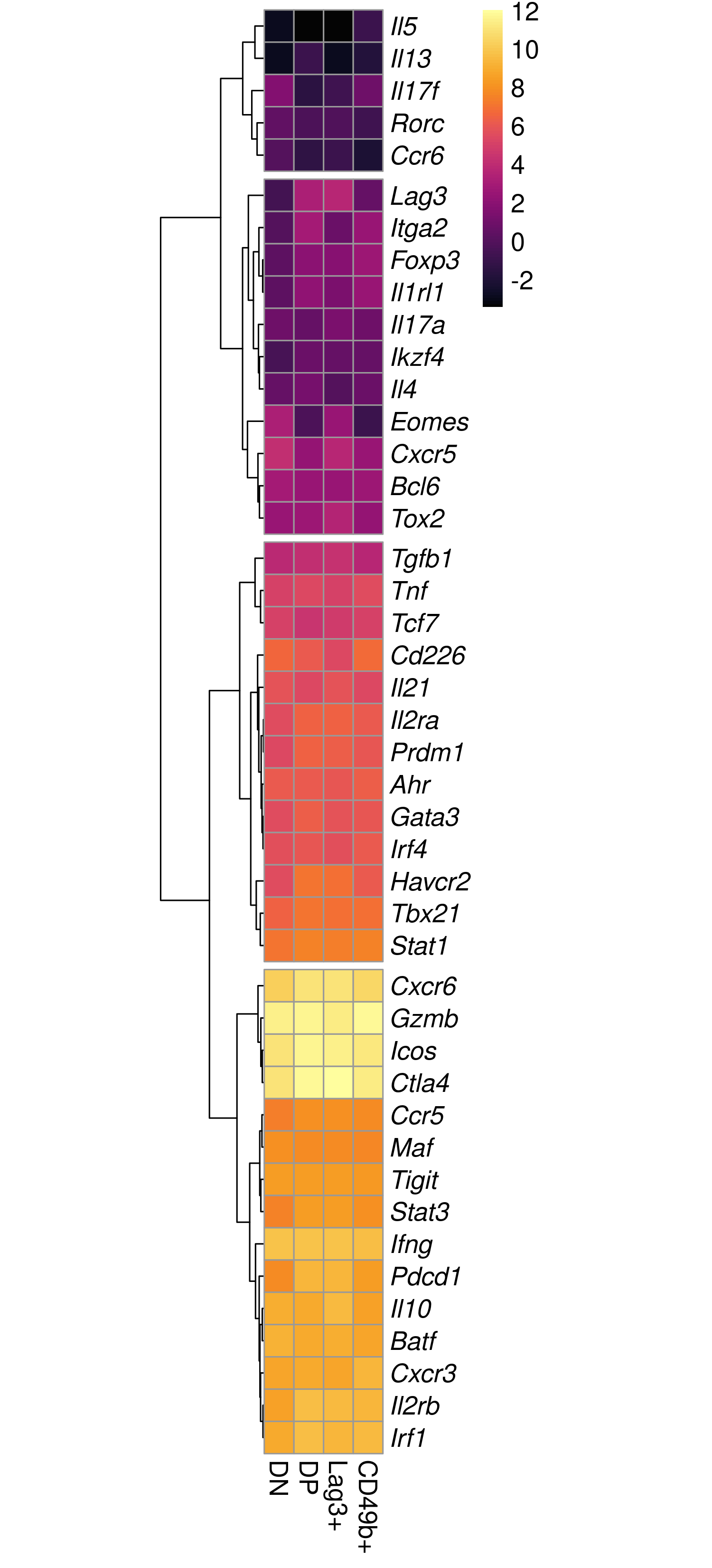

Expression patterns across all groups for key marker genes. The same figure is available here as a pdf.

Top 100

All DE genes were combined across all comparisons and the 100 with the most extreme estimates of logFC were chosen for visualisation.

top_100 <- top_tables %>% 
  lapply(dplyr::filter, DE) %>% 
  bind_rows(.id = "comparison") %>% 
  arrange(desc(abs(logFC))) %>% 
  distinct(gene_id) %>% 
  dplyr::slice(1:100) %>% 
  pull("gene_id")
p <- grp_coef[top_100,] %>% 
  # t() %>% 
  pheatmap(
    color = hcl.colors(101, "inferno"),
    labels_row = id2gene[top_100],
    labels_col = c(DN = "DN", DP = "DP", "LAG_3" = "Lag3+", CD49b = "Cd49b+"),
    cluster_cols = FALSE,
    # annotation_col = top_tables %>%
    #   lapply(
    #     function(x) {
    #       up <- dplyr::filter(x, DE, logFC > 0)$gene_id
    #       down <- dplyr::filter(x, DE, logFC < 0)$gene_id
    #       case_when(
    #         top_100 %in% up ~ "Up",
    #         top_100 %in% down ~ "Down",
    #         TRUE ~ "Unchanged"
    #       )
    #     }
    #   ) %>%
    #   lapply(factor, levels = c("Up", "Down", "Unchanged")) %>%
    #   as.data.frame() %>%
    #   set_colnames(str_replace_all(colnames(.), "v", " Vs. ")) %>%
    #   set_rownames(top_100),
    # annotation_colors = top_tables %>%
    #   setNames(str_replace_all(names(.), "v", " Vs. ")) %>%
    #   lapply(function(x) c("Unchanged" = "grey", "Up" = "red", "Down" = "blue")),
    # annotation_legend = FALSE,
    cutree_rows = 8,
    cellwidth = 15,
    fontsize = 9,
    silent = TRUE
  ) %>% 
  .[["gtable"]]
p$grobs[[4]]$gp <- gpar(fontsize = 9, fontface = "italic")
p$grobs[[3]]$gp <- gpar(fontsize = 10)
png(
  here::here("docs", "assets", "top100_heat.png"),
  height = 12, width = 5, units = "in", res = 300
)
grid.newpage()
grid.draw(p)
dev.off()
pdf(
  here::here("docs", "assets", "top100_heat.pdf"),
  height = 12, width = 5
)
grid.newpage()
grid.draw(p)
dev.off()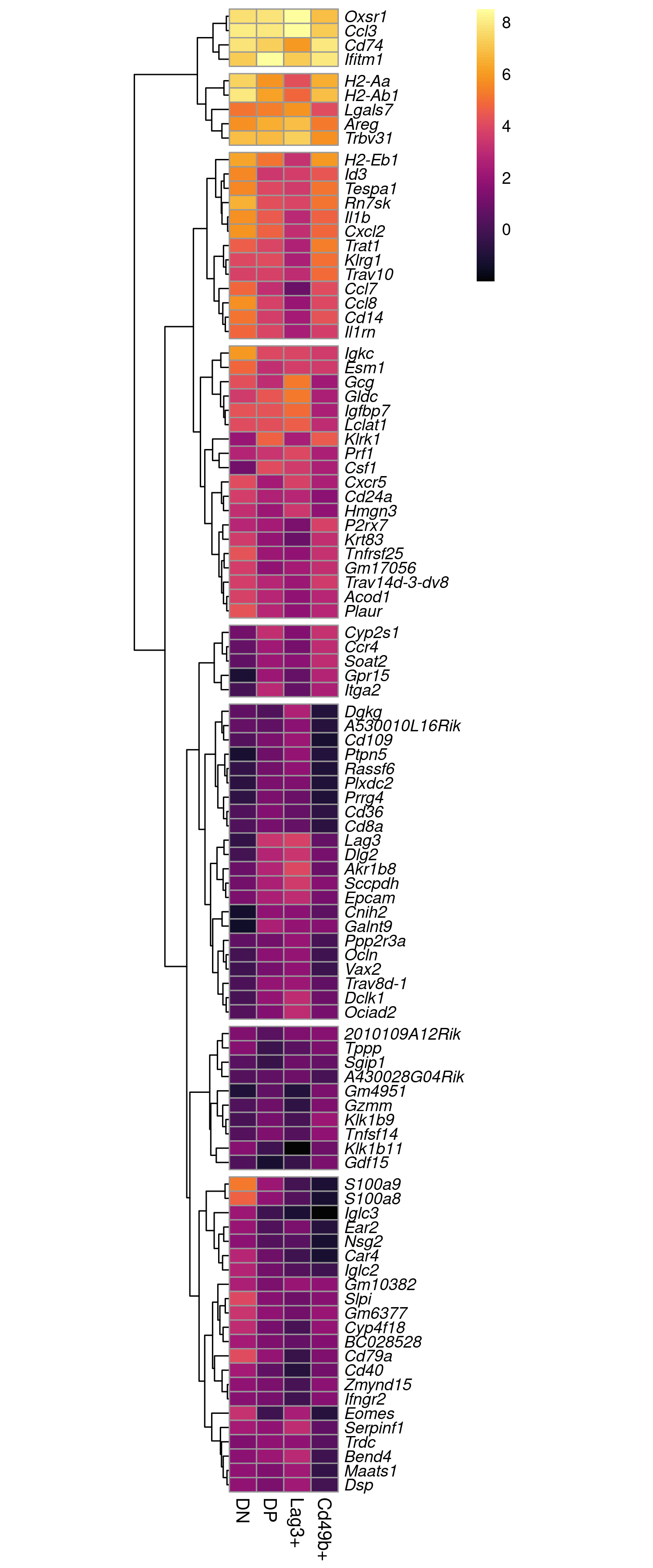

Expression patterns the top 100 DE genes by logFC. The same figure is available here as a pdf.

Top 100 By logFC

n <- 101
myPalette <- colorRampPalette(c("blue", "white", "red"))(n)
myBreaks <- c(
  seq(-7, -7/n, length.out = (n - 1) / 2), 
  0,
  seq(9 / n, 9, length.out = (n - 1) / 2)
)
p <- fit$coefficients[top_100,c(1:4, 6, 5)] %>% 
  pheatmap(
    color = myPalette,
    breaks = myBreaks,
    legend_breaks = seq(-6, 8, by = 2),
    cellwidth = 15,
    labels_row = id2gene[top_100],
    cutree_rows = 5,
    fontsize = 9,
    cluster_cols = FALSE,
    labels_col = setNames(
      str_replace(colnames(.), "v", " Vs. "),
      colnames(.)
    ),
    silent = TRUE
  ) %>% 
  .[["gtable"]]
p$grobs[[4]]$gp <- gpar(fontface = "italic")
png(
  here::here("docs", "assets", "top100_logfc_heat.png"),
  height = 12, width = 5, units = "in", res = 300
)
grid.newpage()
grid.draw(p)
dev.off()
pdf(
  here::here("docs", "assets", "top100_logfc_heat.pdf"),
  height = 12, width = 5
)
grid.newpage()
grid.draw(p)
dev.off()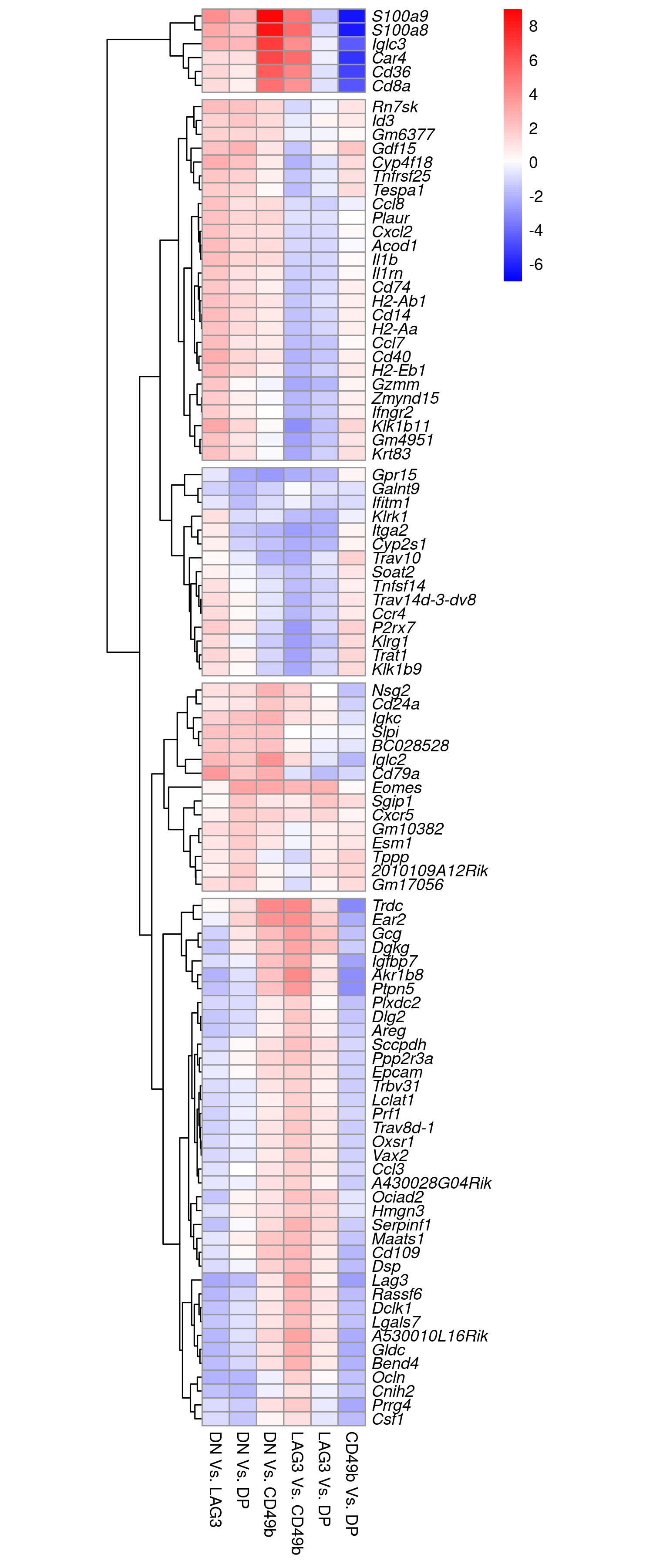

Changes in relative expression for the top 100 DE genes by logFC. The same figure is available here as a pdf.

Data Export

write_rds(dgeFilt, here::here("output", "dgeFilt.rds"), compress = "gz")
write_rds(top_tables, here::here("output", "top_tables.rds"), compress = "gz")
write_rds(v, here::here("output", "v.rds"), compress = "gz")
write_rds(fit, here::here("output", "fit.rds"), compress = "gz")

sessionInfo()

R version 4.3.0 (2023-04-21)
Platform: x86_64-pc-linux-gnu (64-bit)
Running under: Ubuntu 20.04.6 LTS

Matrix products: default
BLAS:   /usr/lib/x86_64-linux-gnu/blas/libblas.so.3.9.0 
LAPACK: /usr/lib/x86_64-linux-gnu/lapack/liblapack.so.3.9.0

locale:
 [1] LC_CTYPE=en_AU.UTF-8       LC_NUMERIC=C              
 [3] LC_TIME=en_AU.UTF-8        LC_COLLATE=en_AU.UTF-8    
 [5] LC_MONETARY=en_AU.UTF-8    LC_MESSAGES=en_AU.UTF-8   
 [7] LC_PAPER=en_AU.UTF-8       LC_NAME=C                 
 [9] LC_ADDRESS=C               LC_TELEPHONE=C            
[11] LC_MEASUREMENT=en_AU.UTF-8 LC_IDENTIFICATION=C       

time zone: Australia/Adelaide
tzcode source: system (glibc)

attached base packages:
[1] grid      stats4    stats     graphics  grDevices utils     datasets 
[8] methods   base     

other attached packages:
 [1] reactable_0.4.4         ComplexUpset_1.3.3      pander_0.6.5           
 [4] glue_1.6.2              broom_1.0.4             scales_1.2.1           
 [7] ensembldb_2.24.0        AnnotationFilter_1.24.0 GenomicFeatures_1.52.0 
[10] AnnotationDbi_1.62.0    Biobase_2.60.0          GenomicRanges_1.52.0   
[13] GenomeInfoDb_1.36.0     IRanges_2.34.0          S4Vectors_0.38.0       
[16] AnnotationHub_3.8.0     BiocFileCache_2.8.0     dbplyr_2.3.2           
[19] BiocGenerics_0.46.0     pheatmap_1.0.12         ggrepel_0.9.3          
[22] edgeR_3.42.0            limma_3.56.0            magrittr_2.0.3         
[25] lubridate_1.9.2         forcats_1.0.0           stringr_1.5.0          
[28] dplyr_1.1.2             purrr_1.0.1             readr_2.1.4            
[31] tidyr_1.3.0             tibble_3.2.1            ggplot2_3.4.2          
[34] tidyverse_2.0.0         workflowr_1.7.0        

loaded via a namespace (and not attached):
  [1] RColorBrewer_1.1-3            rstudioapi_0.14              
  [3] jsonlite_1.8.4                farver_2.1.1                 
  [5] rmarkdown_2.21                fs_1.6.2                     
  [7] BiocIO_1.10.0                 zlibbioc_1.46.0              
  [9] vctrs_0.6.2                   memoise_2.0.1                
 [11] Rsamtools_2.16.0              RCurl_1.98-1.12              
 [13] htmltools_0.5.5               progress_1.2.2               
 [15] curl_5.0.0                    sass_0.4.5                   
 [17] bslib_0.4.2                   htmlwidgets_1.6.2            
 [19] cachem_1.0.7                  GenomicAlignments_1.36.0     
 [21] whisker_0.4.1                 mime_0.12                    
 [23] lifecycle_1.0.3               pkgconfig_2.0.3              
 [25] Matrix_1.5-4                  R6_2.5.1                     
 [27] fastmap_1.1.1                 GenomeInfoDbData_1.2.10      
 [29] MatrixGenerics_1.12.0         shiny_1.7.4                  
 [31] digest_0.6.31                 colorspace_2.1-0             
 [33] patchwork_1.1.2               ps_1.7.5                     
 [35] rprojroot_2.0.3               RSQLite_2.3.1                
 [37] labeling_0.4.2                filelock_1.0.2               
 [39] fansi_1.0.4                   timechange_0.2.0             
 [41] mgcv_1.8-42                   httr_1.4.5                   
 [43] compiler_4.3.0                here_1.0.1                   
 [45] bit64_4.0.5                   withr_2.5.0                  
 [47] backports_1.4.1               BiocParallel_1.34.0          
 [49] DBI_1.1.3                     highr_0.10                   
 [51] biomaRt_2.56.0                rappdirs_0.3.3               
 [53] DelayedArray_0.25.0           rjson_0.2.21                 
 [55] tools_4.3.0                   interactiveDisplayBase_1.38.0
 [57] httpuv_1.6.9                  restfulr_0.0.15              
 [59] callr_3.7.3                   nlme_3.1-162                 
 [61] promises_1.2.0.1              getPass_0.2-2                
 [63] generics_0.1.3                gtable_0.3.3                 
 [65] tzdb_0.3.0                    hms_1.1.3                    
 [67] xml2_1.3.4                    utf8_1.2.3                   
 [69] XVector_0.40.0                BiocVersion_3.17.1           
 [71] pillar_1.9.0                  vroom_1.6.1                  
 [73] later_1.3.0                   splines_4.3.0                
 [75] lattice_0.21-8                rtracklayer_1.60.0           
 [77] bit_4.0.5                     tidyselect_1.2.0             
 [79] locfit_1.5-9.7                Biostrings_2.68.0            
 [81] knitr_1.42                    git2r_0.32.0                 
 [83] ProtGenerics_1.32.0           SummarizedExperiment_1.30.0  
 [85] xfun_0.39                     statmod_1.5.0                
 [87] matrixStats_0.63.0            stringi_1.7.12               
 [89] lazyeval_0.2.2                yaml_2.3.7                   
 [91] evaluate_0.20                 codetools_0.2-19             
 [93] BiocManager_1.30.20           cli_3.6.1                    
 [95] xtable_1.8-4                  munsell_0.5.0                
 [97] processx_3.8.1                jquerylib_0.1.4              
 [99] Rcpp_1.0.10                   png_0.1-8                    
[101] XML_3.99-0.14                 parallel_4.3.0               
[103] ellipsis_0.3.2                blob_1.2.4                   
[105] prettyunits_1.1.1             bitops_1.0-7                 
[107] crayon_1.5.2                  rlang_1.1.0                  
[109] KEGGREST_1.40.0

Tr1: Differential Gene Expression

Stephen Pederson & Caitlin Abbott

02 May, 2023

Data Preparation & Inspection

Library Sizes

Count Densities

PCA

Model Fitting

Summary Table

MA Plots

DN Vs. LAG3

DN Vs. DP

DN Vs. CD49b

LAG3 Vs. CD49b

LAG3 Vs. DP

CD49b Vs. DP

Volcano Plots

DN Vs. LAG3

DN Vs. DP

DN Vs. CD49b

LAG3 Vs. CD49b

LAG3 Vs. DP

CD49b Vs. DP

DE Gene Summary

UpSet Plot

Heatmaps

Key Signatures

High Confidence Genes

Top 100

Top 100 By logFC

Data Export