Tr1: Enrichment Analysis
Stephen Pederson & Caitlin Abbott
01 May, 2023
Last updated: 2023-05-01
Checks: 6 1
Knit directory: Tr1-RNA-Sequencing-/
This reproducible R Markdown analysis was created with workflowr (version 1.7.0). The Checks tab describes the reproducibility checks that were applied when the results were created. The Past versions tab lists the development history.
The R Markdown file has unstaged changes. To know which version of
the R Markdown file created these results, you’ll want to first commit
it to the Git repo. If you’re still working on the analysis, you can
ignore this warning. When you’re finished, you can run
wflow_publish to commit the R Markdown file and build the
HTML.
Great job! The global environment was empty. Objects defined in the global environment can affect the analysis in your R Markdown file in unknown ways. For reproduciblity it’s best to always run the code in an empty environment.
The command set.seed(20221025) was run prior to running
the code in the R Markdown file. Setting a seed ensures that any results
that rely on randomness, e.g. subsampling or permutations, are
reproducible.
Great job! Recording the operating system, R version, and package versions is critical for reproducibility.
Nice! There were no cached chunks for this analysis, so you can be confident that you successfully produced the results during this run.
Great job! Using relative paths to the files within your workflowr project makes it easier to run your code on other machines.
Great! You are using Git for version control. Tracking code development and connecting the code version to the results is critical for reproducibility.
The results in this page were generated with repository version ef7ce0c. See the Past versions tab to see a history of the changes made to the R Markdown and HTML files.
Note that you need to be careful to ensure that all relevant files for
the analysis have been committed to Git prior to generating the results
(you can use wflow_publish or
wflow_git_commit). workflowr only checks the R Markdown
file, but you know if there are other scripts or data files that it
depends on. Below is the status of the Git repository when the results
were generated:
Ignored files:
    Ignored:    .Rhistory
    Ignored:    .Rproj.user/

Unstaged changes:
    Modified:   analysis/enrichment.Rmd
Note that any generated files, e.g. HTML, png, CSS, etc., are not included in this status report because it is ok for generated content to have uncommitted changes.
These are the previous versions of the repository in which changes were
made to the R Markdown (analysis/enrichment.Rmd) and HTML
(docs/enrichment.html) files. If you’ve configured a remote
Git repository (see ?wflow_git_remote), click on the
hyperlinks in the table below to view the files as they were in that
past version.
| File | Version | Author | Date | Message |
|---|---|---|---|---|
| Rmd | 3933b92 | steveped | 2022-11-18 | Corrected section ids |
| html | 3933b92 | steveped | 2022-11-18 | Corrected section ids |
| html | 3a59bc5 | steveped | 2022-11-18 | Build site. |
| Rmd | 36a1cb8 | steveped | 2022-11-18 | Added enrichment tables |
| html | 0b3ca1b | steveped | 2022-11-17 | Build site. |
| Rmd | 68c392f | steveped | 2022-11-17 | Added down & up genes separately |
| html | f2ee30e | steveped | 2022-11-14 | Build site. |
| Rmd | 61ec31f | Steve Pederson | 2022-11-01 | Added enrichment testing |
| html | 61ec31f | Steve Pederson | 2022-11-01 | Added enrichment testing |
| Rmd | 0892674 | Steve Pederson | 2022-10-26 | Started adding heatmaps |
| Rmd | 8745ba2 | Steve Pederson | 2022-10-26 | Shifted to workflowr |
knitr::opts_chunk$set(
  warning = FALSE, message = FALSE,
  fig.width = 10, fig.height = 8,
  dev = c("png", "pdf")
)
library(tidyverse)
library(limma)
library(edgeR)
library(RColorBrewer)
library(pheatmap)
library(magrittr)
library(clusterProfiler)
library(org.Mm.eg.db)
library(reactable)
library(htmltools)
library(glue)
library(scales)
with_tooltip <- function(value, width = 30) {
tags$span(title = value, str_trunc(value, width))
}top_tables <- read_rds(here::here("output", "top_tables.rds"))
dgeFilt <- read_rds(here::here("output", "dgeFilt.rds"))universe <- dgeFilt$genes$entrezid %>%
unlist() %>%
extract(!is.na(.)) %>% #keep non NA gene
unique() %>%
as.character()Enrichment Results
ego_results <- top_tables %>%
lapply(
function(x) {
de <- dplyr::filter(x, adj.P.Val < 0.05, abs(logFC) > 1)
ids <- unique(unlist(de$entrezid))
enrichGO(
ids,
universe = universe,
OrgDb = org.Mm.eg.db,
ont = "ALL",
keyType = "ENTREZID",
pAdjustMethod = "bonferroni",
pvalueCutoff = 0.05,
qvalueCutoff = 0.05,
readable = TRUE
)
}
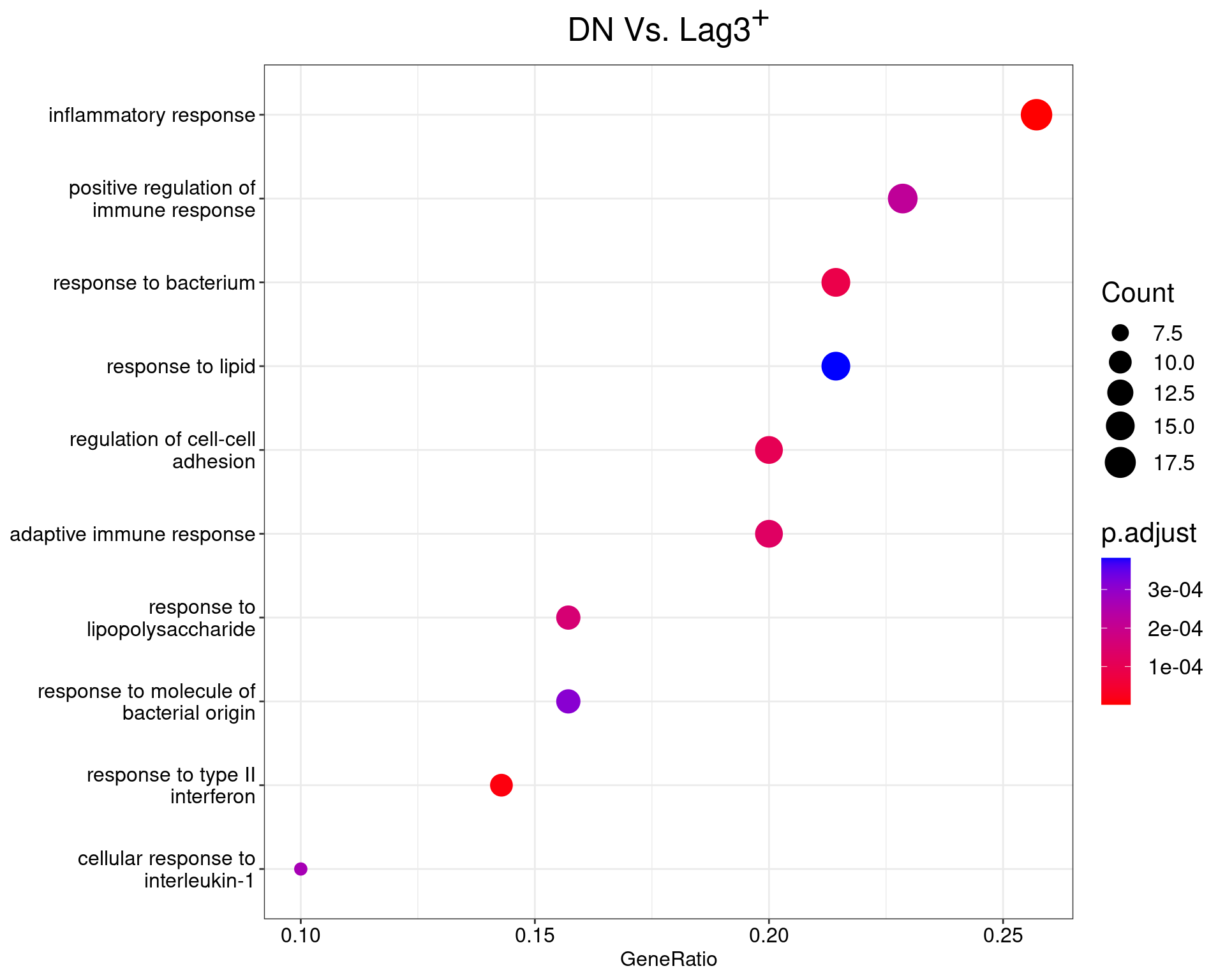
)Enrichment testing was performed using all three available Gene
Ontologies and the function enrichGO() from the package
clusterProfiler. Ontologies were only considered to be
enriched amongst the differentially expressed genes if a
Bonferroni-adjusted p-value < 0.05 was returned during enrichment
testing, with no regard to the sign of fold change.
DN Vs. Lag3+
dotplot(ego_results$DNvLAG3) +
  ggtitle(expression(paste("DN Vs. Lag", 3^{textstyle("+")}))) +
  scale_y_discrete(labels = label_wrap(25)) +
  theme(
    plot.title = element_text(hjust = 0.5),
    text = element_text(size = 16)
  )
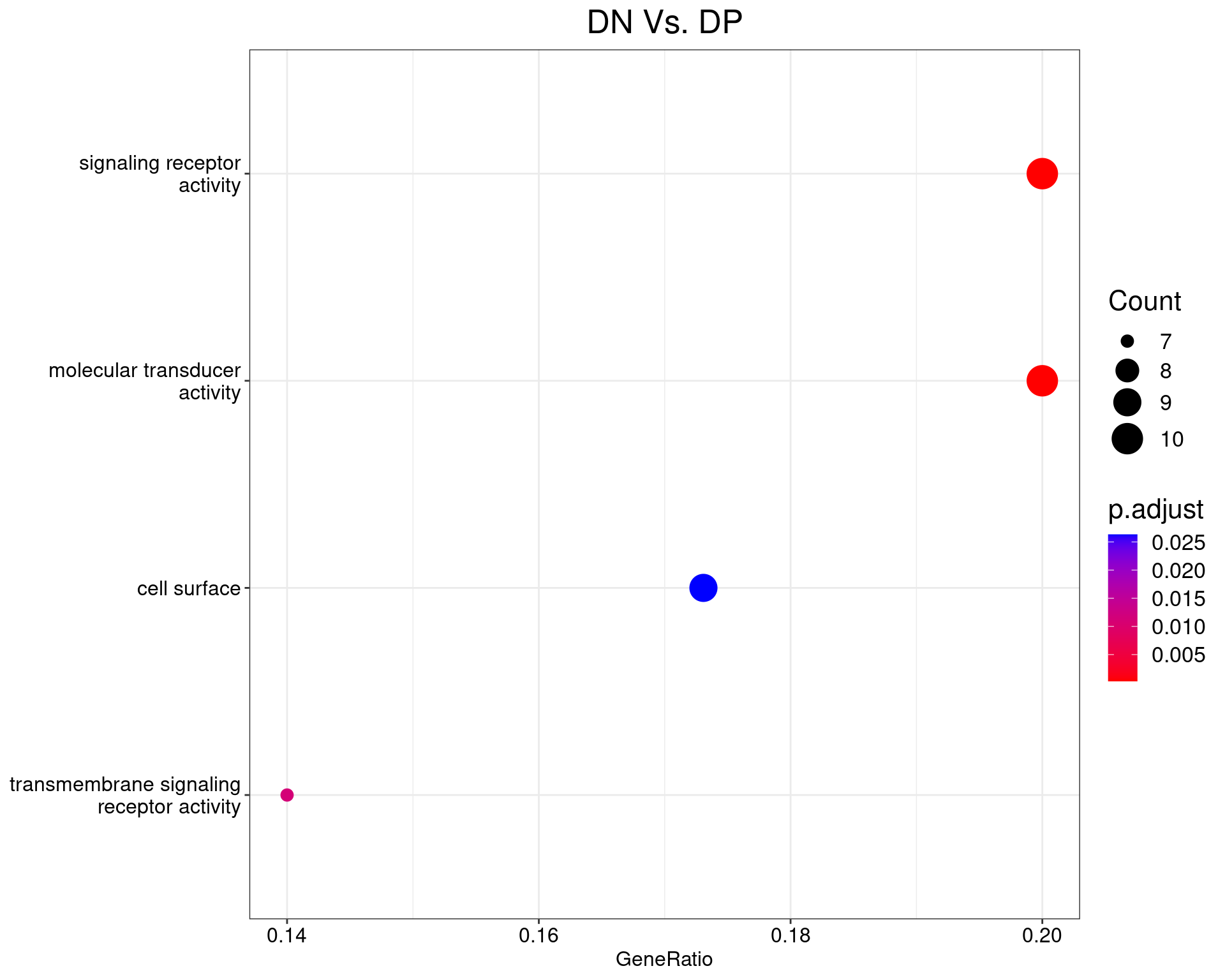
DN Vs. DP
dotplot(ego_results$DNvDP) +
  ggtitle("DN Vs. DP") +
  scale_y_discrete(labels = label_wrap(25)) +
  theme(
    plot.title = element_text(hjust = 0.5),
    text = element_text(size = 16)
  )
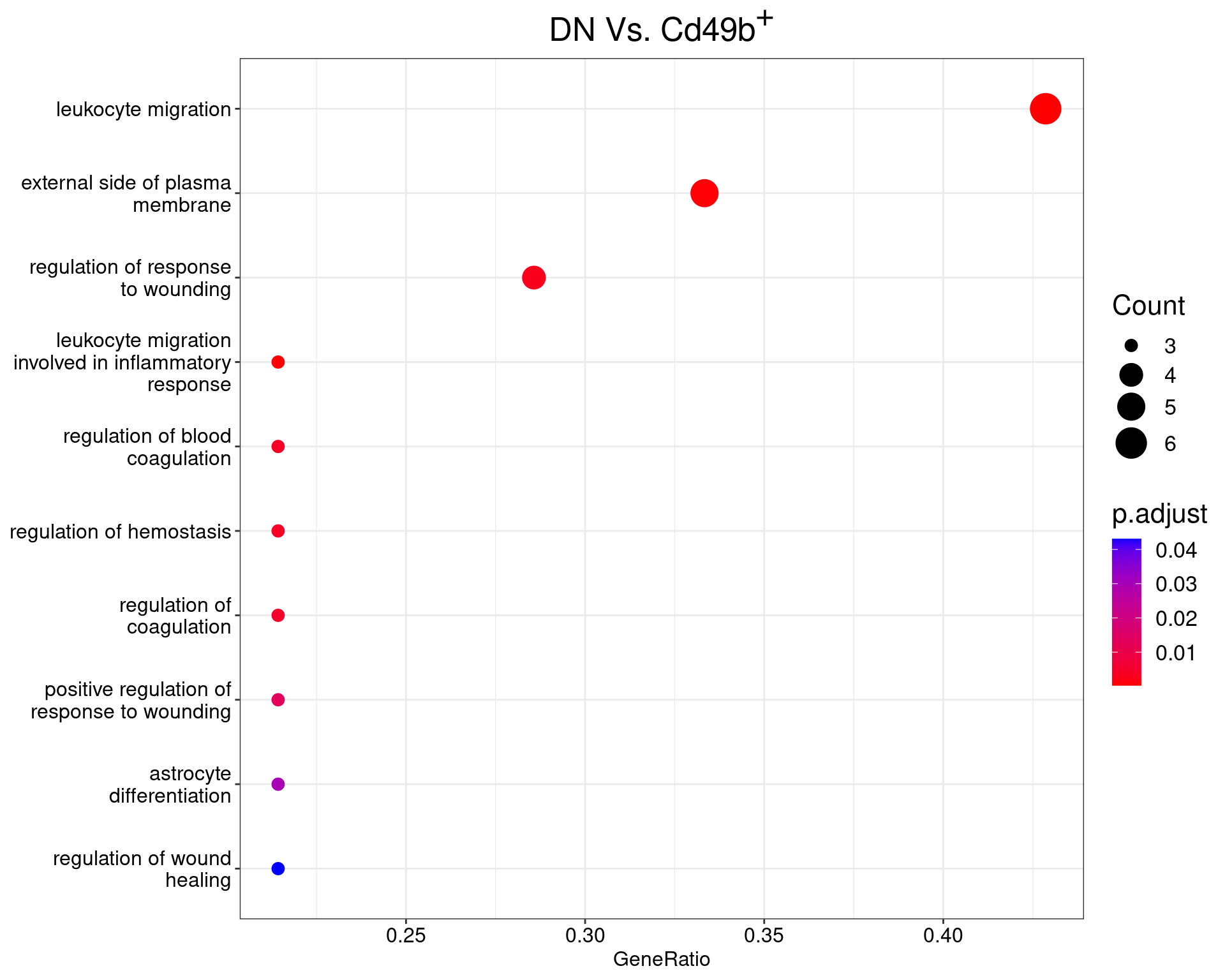
DN Vs. Cd49b+
dotplot(ego_results$DNvCD49b) +
  ggtitle(expression(paste("DN Vs. Cd49", b^{textstyle("+")}))) +
  scale_y_discrete(labels = label_wrap(25)) +
  theme(
    plot.title = element_text(hjust = 0.5),
    text = element_text(size = 16)
  )
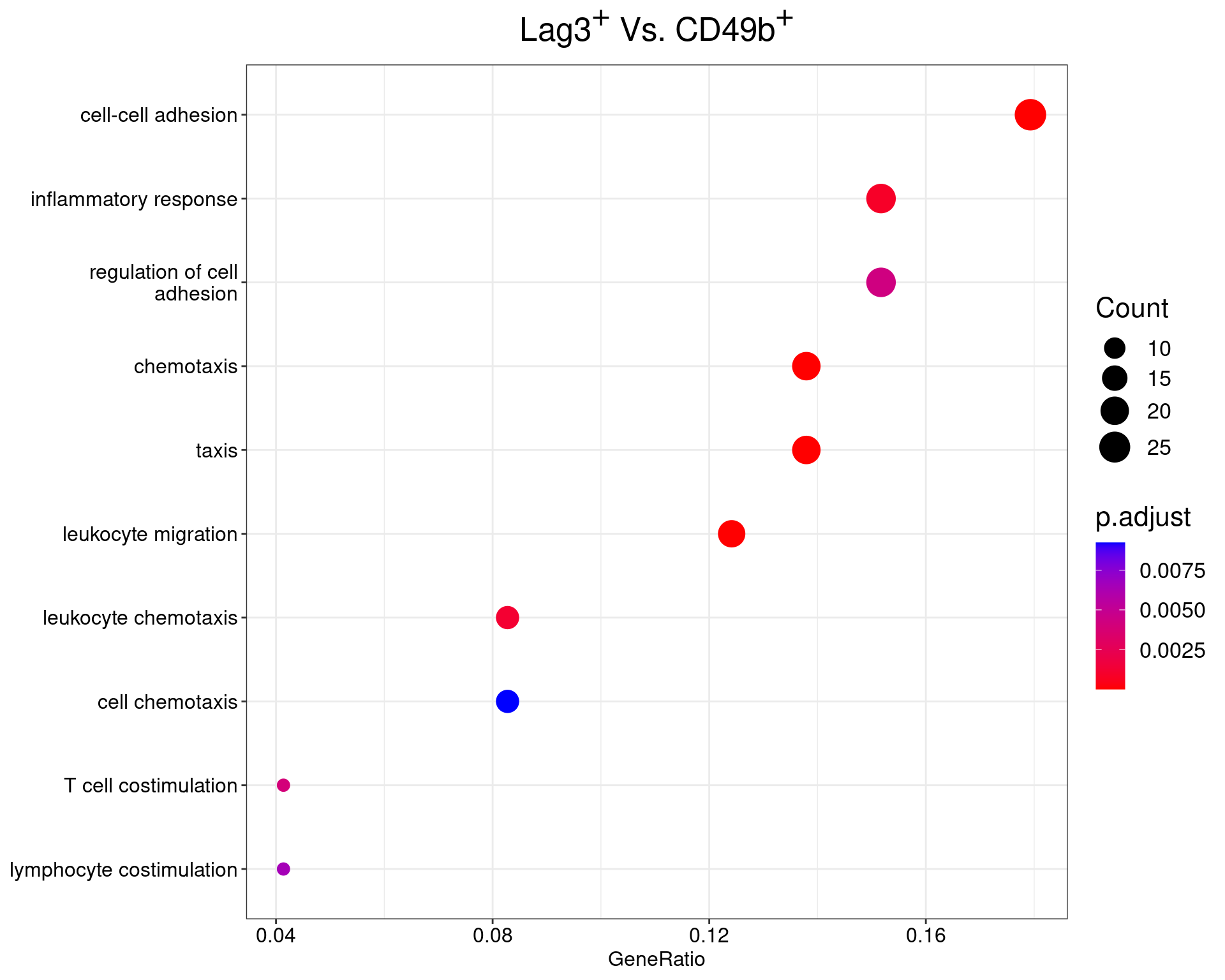
Lag3+ Vs Cd49+
dotplot(ego_results$LAG3vCD49b) +
  ggtitle(
    expression(
      paste("Lag", 3^{textstyle("+")}, " Vs. CD49", b^{textstyle("+")})
    )
  ) +
  scale_y_discrete(labels = label_wrap(25)) +
  theme(
    plot.title = element_text(hjust = 0.5),
    text = element_text(size = 16)
  )
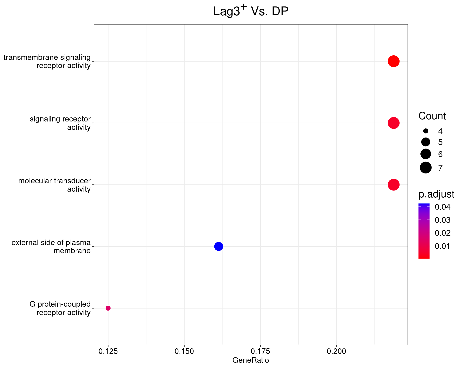
Lag3+ Vs. DP
dotplot(ego_results$LAG3vDP) +
  ggtitle(expression(paste("Lag", 3^{textstyle("+")}, " Vs. DP"))) +
  scale_y_discrete(labels = label_wrap(25)) +
  theme(
    plot.title = element_text(hjust = 0.5),
    text = element_text(size = 16)
  )
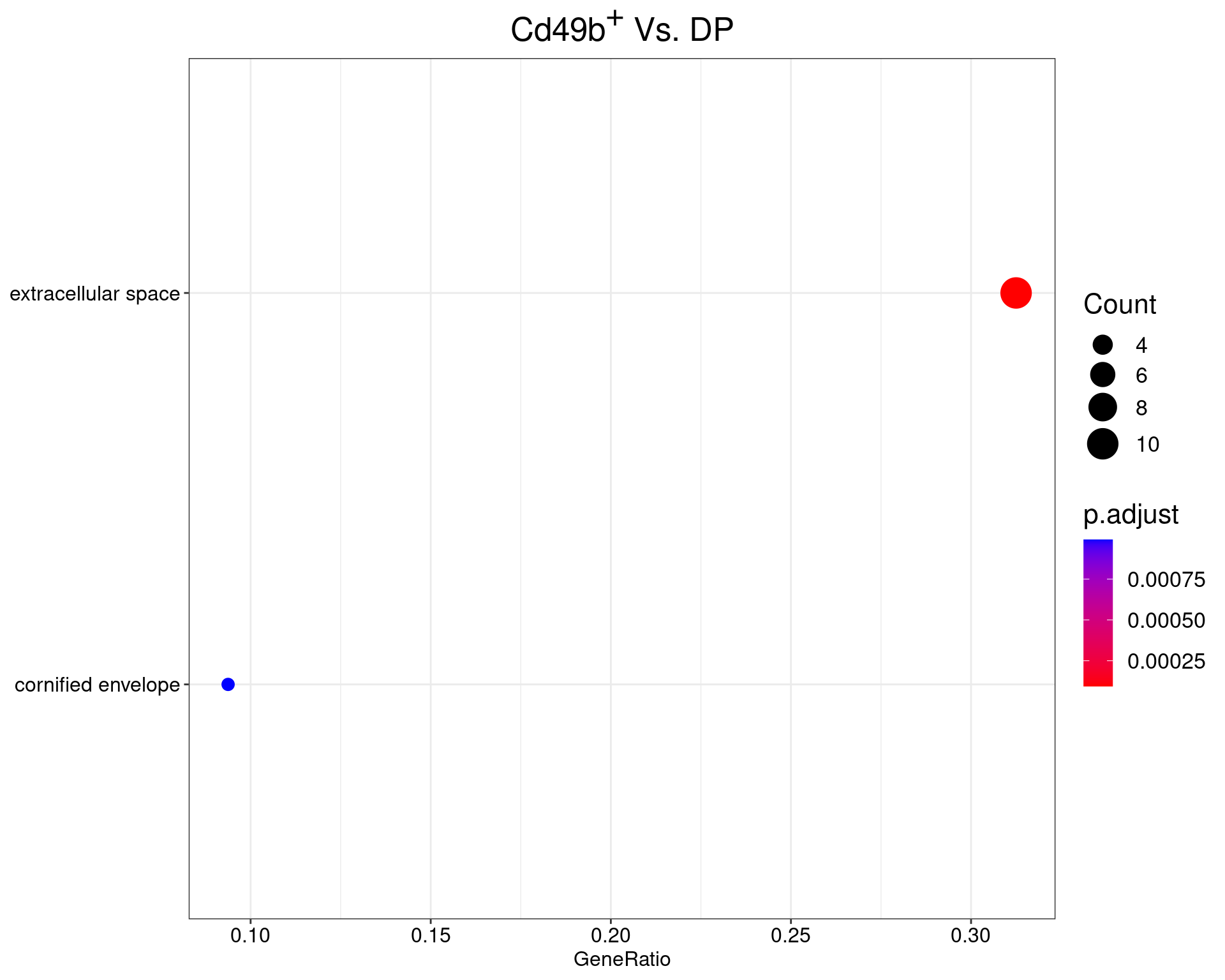
Cd49b+ Vs. DP
dotplot(ego_results$CD49bvDP) +
  ggtitle(expression(paste("Cd49", b^{textstyle("+")}, " Vs. DP"))) +
  scale_y_discrete(labels = label_wrap(25)) +
  theme(
    plot.title = element_text(hjust = 0.5),
    text = element_text(size = 16)
  )
Enrichment Tables
htmltools::tagList(
  names(ego_results) %>%
    lapply(
      function(x) {
        df <- ego_results[[x]] %>%
          as_tibble() %>%
          dplyr::filter(p.adjust < 0.05) %>%
          mutate(
            geneID = str_replace_all(geneID, "\\/", "; "),
            `% DE` = vapply(GeneRatio, function(x) eval(parse(text = x)), numeric(1)),
            `% BG` = vapply(BgRatio, function(x) eval(parse(text = x)), numeric(1))
          ) %>%
          dplyr::select(ONTOLOGY, ID, Description, Count, starts_with("%"), p.adjust, geneID) %>%
          arrange(p.adjust) %>%
          distinct(ONTOLOGY, geneID, .keep_all = TRUE)

        if (nrow(df)) {
          cp <- glue(
            "All {nrow(df)} ontologies considered enriched in the set of ",
            length(unique(unlist(dplyr::filter(top_tables[[x]], DE)$entrezid))),
            " DE genes mapped to EntrezIDs from the comparison {x}. Enrichment ",
            "testing was performed using Fisher's Exact Test compared to the set of ",
            comma(length(unique(universe))),
            " unique EntrezIDs mapped to genes considered as detectable. ",
            "The percentage of nonDE genes mapped to the ontology are also given. ",
            "P-values are Bonferroni adjusted and all pathways are considered enriched ",
            "using an adjusted p-value < 0.05. In order to see all DE genes, hover your ",
            "mouse over the final column. ",
            "Where the identical genes map to multiple terms within each ontology, only ",
            "the term with the lowest p-value (i.e. strongest enrichment) is shown. ",
            "As a result, some of the pathways seen in the above dotplots may not be ",
            "presented in these tables."
          )
          htmltools::div(
            htmltools::div(
              id = x,
              class="section level3",
              htmltools::h3(class = "tabset", x),
              htmltools::tags$em(cp),
              df %>%
                reactable(
                  filterable = TRUE,
                  columns = list(
                    ONTOLOGY = colDef(name = "Ontology", maxWidth = 100),
                    ID = colDef(name = "GO ID", maxWidth = 125),
                    Description = colDef(maxWidth = 250),
                    Count = colDef(name = "N<sub>DE</sub>", html = TRUE, maxWidth = 80),
                    `% DE` = colDef(format = colFormat(percent = TRUE, digits = 1), maxWidth = 85),
                    `% BG` = colDef(format = colFormat(percent = TRUE, digits = 1), maxWidth = 85),
                    p.adjust = colDef(
                      name = "p<sub>adj</sub>", html = TRUE, maxWidth = 100,
                      cell = function(value) {
                        fm <- ifelse(value < 0.001, "%.2e", "%.3f")
                        sprintf(fm, value)
                      }
                    ),
                    geneID = colDef(
                      name = "DE Genes",
                      cell = function(value) with_tooltip(value, width = 100)
                    )
                  )
                )
            )
          )
        } else {
          cat(glue("No enrichment was found for {x}\n\n"))
        }
      }
    )
)
DNvLAG3
All 55 ontologies considered enriched in the set of 73 DE genes mapped to EntrezIDs from the comparison DNvLAG3. Enrichment testing was performed using Fisher's Exact Test compared to the set of 10,006 unique EntrezIDs mapped to genes considered as detectable. The percentage of nonDE genes mapped to the ontology are also given. P-values are Bonferroni adjusted and all pathways are considered enriched using an adjusted p-value < 0.05. In order to see all DE genes, hover your mouse over the final column. Where the identical genes map to multiple terms within each ontology, only the term with the lowest p-value (i.e. strongest enrichment) is shown. As a result, some of the pathways seen in the above dotplots may not be presented in these tables.DNvDP
All 3 ontologies considered enriched in the set of 53 DE genes mapped to EntrezIDs from the comparison DNvDP. Enrichment testing was performed using Fisher's Exact Test compared to the set of 10,006 unique EntrezIDs mapped to genes considered as detectable. The percentage of nonDE genes mapped to the ontology are also given. P-values are Bonferroni adjusted and all pathways are considered enriched using an adjusted p-value < 0.05. In order to see all DE genes, hover your mouse over the final column. Where the identical genes map to multiple terms within each ontology, only the term with the lowest p-value (i.e. strongest enrichment) is shown. As a result, some of the pathways seen in the above dotplots may not be presented in these tables.DNvCD49b
All 10 ontologies considered enriched in the set of 16 DE genes mapped to EntrezIDs from the comparison DNvCD49b. Enrichment testing was performed using Fisher's Exact Test compared to the set of 10,006 unique EntrezIDs mapped to genes considered as detectable. The percentage of nonDE genes mapped to the ontology are also given. P-values are Bonferroni adjusted and all pathways are considered enriched using an adjusted p-value < 0.05. In order to see all DE genes, hover your mouse over the final column. Where the identical genes map to multiple terms within each ontology, only the term with the lowest p-value (i.e. strongest enrichment) is shown. As a result, some of the pathways seen in the above dotplots may not be presented in these tables.LAG3vCD49b
All 36 ontologies considered enriched in the set of 151 DE genes mapped to EntrezIDs from the comparison LAG3vCD49b. Enrichment testing was performed using Fisher's Exact Test compared to the set of 10,006 unique EntrezIDs mapped to genes considered as detectable. The percentage of nonDE genes mapped to the ontology are also given. P-values are Bonferroni adjusted and all pathways are considered enriched using an adjusted p-value < 0.05. In order to see all DE genes, hover your mouse over the final column. Where the identical genes map to multiple terms within each ontology, only the term with the lowest p-value (i.e. strongest enrichment) is shown. As a result, some of the pathways seen in the above dotplots may not be presented in these tables.CD49bvDP
All 2 ontologies considered enriched in the set of 33 DE genes mapped to EntrezIDs from the comparison CD49bvDP. Enrichment testing was performed using Fisher's Exact Test compared to the set of 10,006 unique EntrezIDs mapped to genes considered as detectable. The percentage of nonDE genes mapped to the ontology are also given. P-values are Bonferroni adjusted and all pathways are considered enriched using an adjusted p-value < 0.05. In order to see all DE genes, hover your mouse over the final column. Where the identical genes map to multiple terms within each ontology, only the term with the lowest p-value (i.e. strongest enrichment) is shown. As a result, some of the pathways seen in the above dotplots may not be presented in these tables.LAG3vDP
All 3 ontologies considered enriched in the set of 33 DE genes mapped to EntrezIDs from the comparison LAG3vDP. Enrichment testing was performed using Fisher's Exact Test compared to the set of 10,006 unique EntrezIDs mapped to genes considered as detectable. The percentage of nonDE genes mapped to the ontology are also given. P-values are Bonferroni adjusted and all pathways are considered enriched using an adjusted p-value < 0.05. In order to see all DE genes, hover your mouse over the final column. Where the identical genes map to multiple terms within each ontology, only the term with the lowest p-value (i.e. strongest enrichment) is shown. As a result, some of the pathways seen in the above dotplots may not be presented in these tables.Enrichment Results (Up Only)
ego_results <- top_tables %>%
lapply(
function(x) {
de <- dplyr::filter(x, adj.P.Val < 0.05, logFC > 1)
ids <- unique(unlist(de$entrezid))
enrichGO(
ids,
universe = universe,
OrgDb = org.Mm.eg.db,
ont = "ALL",
keyType = "ENTREZID",
pAdjustMethod = "bonferroni",
pvalueCutoff = 0.05,
qvalueCutoff = 0.05,
readable = TRUE
)
}
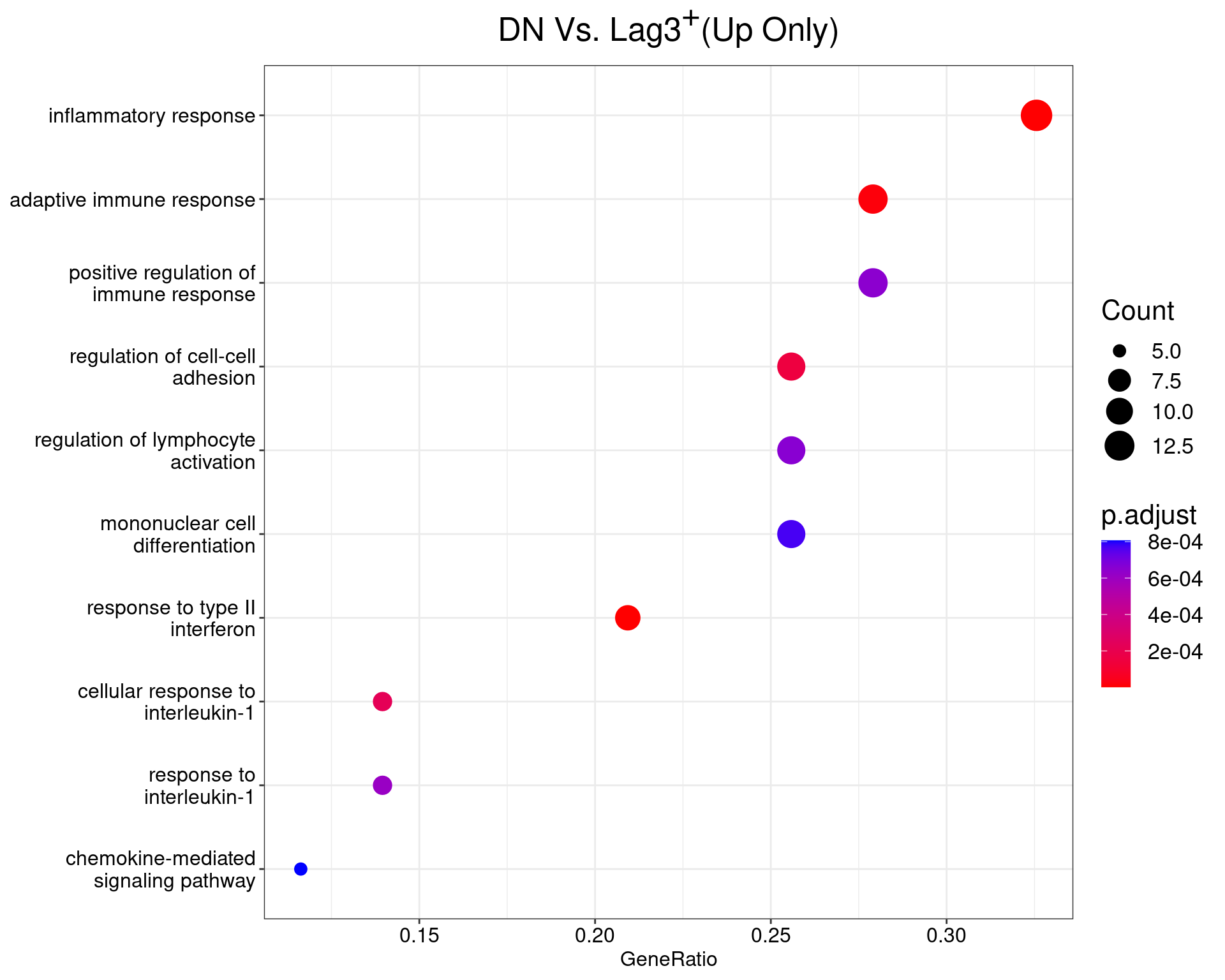
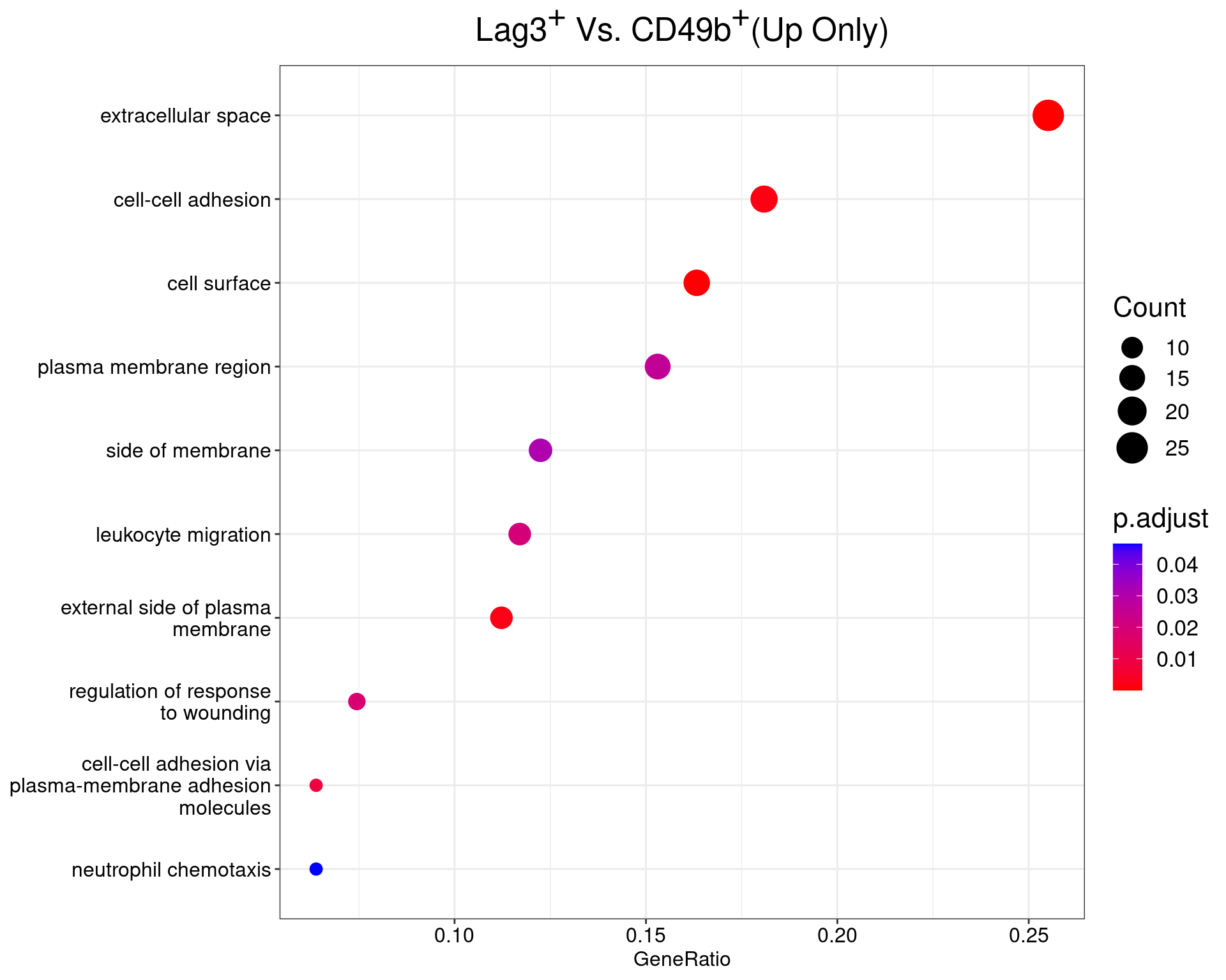
)Enrichment testing was repeated using all three available Gene
Ontologies and the function enrichGO() from the package
clusterProfiler. Ontologies were only considered to be
enriched amongst the up-regulated genes if a
Bonferroni-adjusted p-value < 0.05 was returned during enrichment
testing. Please note that an up-regulated gene does not always
correspond to an increase in activity of a pathway.
DN Vs. Lag3+
dotplot(ego_results$DNvLAG3) +
  ggtitle(expression(paste("DN Vs. Lag", 3^{textstyle("+")}, "(Up Only)"))) +
  scale_y_discrete(labels = label_wrap(25)) +
  theme(
    plot.title = element_text(hjust = 0.5),
    text = element_text(size = 16)
  )
| Version | Author | Date |
|---|---|---|
| 0b3ca1b | steveped | 2022-11-17 |
DN Vs. DP
No significant results were obtained for up-regulated genes in this comparison.
dotplot(ego_results$DNvDP) +
ggtitle("DN Vs. DP (Up Only)") +
scale_y_discrete(labels = label_wrap(25)) +
theme(
plot.title = element_text(hjust = 0.5),
text = element_text(size = 16)
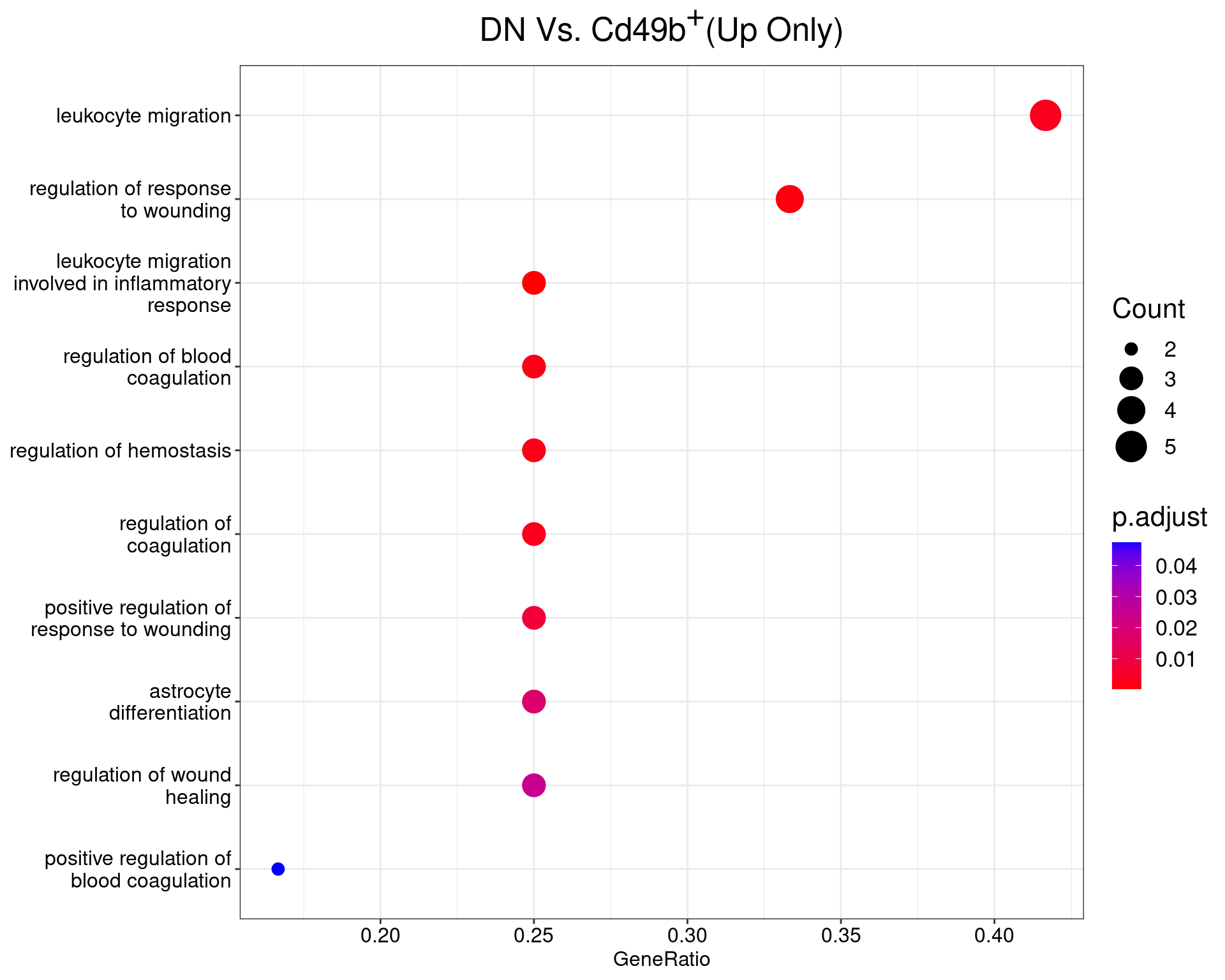
)DN Vs. Cd49b+
dotplot(ego_results$DNvCD49b) +
  ggtitle(expression(paste("DN Vs. Cd49", b^{textstyle("+")}, "(Up Only)"))) +
  scale_y_discrete(labels = label_wrap(25)) +
  theme(
    plot.title = element_text(hjust = 0.5),
    text = element_text(size = 16)
  )
| Version | Author | Date |
|---|---|---|
| 0b3ca1b | steveped | 2022-11-17 |
Lag3+ Vs Cd49+
dotplot(ego_results$LAG3vCD49b) +
  ggtitle(
    expression(
      paste("Lag", 3^{textstyle("+")}, " Vs. CD49", b^{textstyle("+")}, "(Up Only)")
    )
  ) +
  scale_y_discrete(labels = label_wrap(25)) +
  theme(
    plot.title = element_text(hjust = 0.5),
    text = element_text(size = 16)
  )
| Version | Author | Date |
|---|---|---|
| 0b3ca1b | steveped | 2022-11-17 |
Lag3+ Vs. DP
No significant results were obtained for up-regulated genes in this comparison.
dotplot(ego_results$LAG3vDP) +
  ggtitle(expression(paste("Lag", 3^{textstyle("+")}, " Vs. DP", "(Up Only)"))) +
  scale_y_discrete(labels = label_wrap(25)) +
  theme(
    plot.title = element_text(hjust = 0.5),
    text = element_text(size = 16)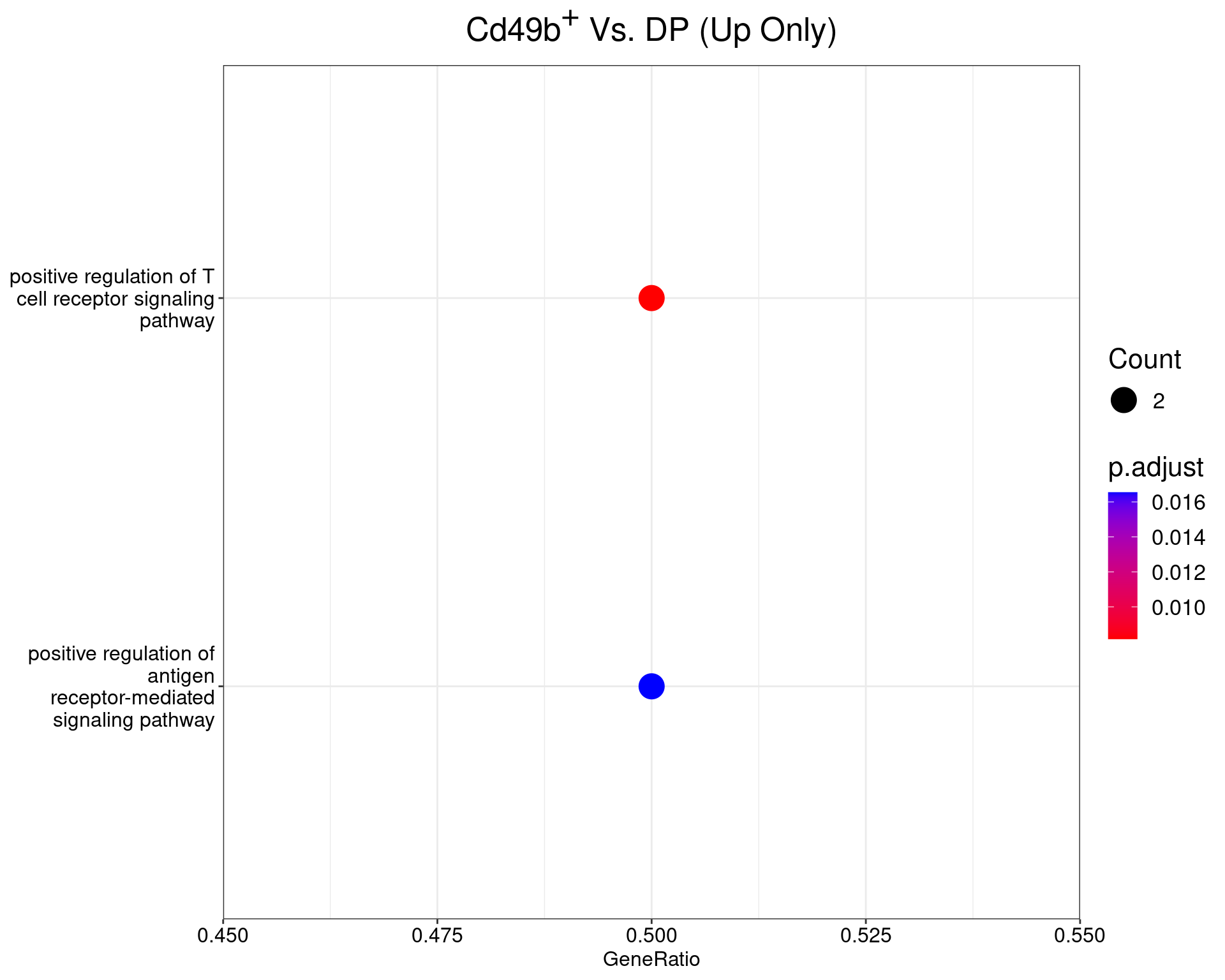
)Cd49b+ Vs. DP
dotplot(ego_results$CD49bvDP) +
  ggtitle(expression(paste("Cd49", b^{textstyle("+")}, " Vs. DP (Up Only)"))) +
  scale_y_discrete(labels = label_wrap(25)) +
  theme(
    plot.title = element_text(hjust = 0.5),
    text = element_text(size = 16)
  )
| Version | Author | Date |
|---|---|---|
| 0b3ca1b | steveped | 2022-11-17 |
Enrichment Tables (Up Only)
ego_results <- ego_results[vapply(ego_results, nrow, integer(1)) > 0]
htmltools::tagList(
  names(ego_results) %>%
    lapply(
      function(x) {
        df <- ego_results[[x]] %>%
          as_tibble() %>%
          dplyr::filter(p.adjust < 0.05) %>%
          mutate(
            geneID = str_replace_all(geneID, "\\/", "; "),
            `% DE` = vapply(GeneRatio, function(x) eval(parse(text = x)), numeric(1)),
            `% BG` = vapply(BgRatio, function(x) eval(parse(text = x)), numeric(1))
          ) %>%
          dplyr::select(ONTOLOGY, ID, Description, Count, starts_with("%"), p.adjust, geneID) %>%
          arrange(p.adjust) %>%
          distinct(ONTOLOGY, geneID, .keep_all = TRUE)

        if (nrow(df)) {
          cp <- glue(
            "All {nrow(df)} ontologies considered enriched in the set of ",
            length(unique(unlist(dplyr::filter(top_tables[[x]], DE, logFC > 1)$entrezid))),
            " up-regulated genes mapped to EntrezIDs from the comparison {x}. Enrichment ",
            "testing was performed using Fisher's Exact Test compared to the set of ",
            comma(length(unique(universe))),
            " unique EntrezIDs mapped to genes considered as detectable. ",
            "The percentage of nonDE genes mapped to the ontology are also given. ",
            "P-values are Bonferroni adjusted and all pathways are considered enriched ",
            "using an adjusted p-value < 0.05. In order to see all DE genes, hover your ",
            "mouse over the final column. ",
            "Where the identical genes map to multiple terms within each ontology, only ",
            "the term with the lowest p-value (i.e. strongest enrichment) is shown. ",
            "As a result, some of the pathways seen in the above dotplots may not be ",
            "presented in these tables."
          )
          htmltools::div(
            htmltools::div(
              id = glue("{x}-up"),
              class="section level3",
              htmltools::h3(class = "tabset", x),
              htmltools::tags$em(cp),
              df %>%
                reactable(
                  filterable = TRUE,
                  columns = list(
                    ONTOLOGY = colDef(name = "Ontology", maxWidth = 100),
                    ID = colDef(name = "GO ID", maxWidth = 125),
                    Description = colDef(maxWidth = 250),
                    Count = colDef(name = "N<sub>DE</sub>", html = TRUE, maxWidth = 80),
                    `% DE` = colDef(format = colFormat(percent = TRUE, digits = 1), maxWidth = 85),
                    `% BG` = colDef(format = colFormat(percent = TRUE, digits = 1), maxWidth = 85),
                    p.adjust = colDef(
                      name = "p<sub>adj</sub>", html = TRUE, maxWidth = 100,
                      cell = function(value) {
                        fm <- ifelse(value < 0.001, "%.2e", "%.3f")
                        sprintf(fm, value)
                      }
                    ),
                    geneID = colDef(
                      name = "DE Genes",
                      cell = function(value) with_tooltip(value, width = 100)
                    )
                  )
                )
            )
          )
        } else {
          cat(glue("No enrichment was found for {x}\n\n"))
        }
      }
    )
)
DNvLAG3
All 55 ontologies considered enriched in the set of 45 up-regulated genes mapped to EntrezIDs from the comparison DNvLAG3. Enrichment testing was performed using Fisher's Exact Test compared to the set of 10,006 unique EntrezIDs mapped to genes considered as detectable. The percentage of nonDE genes mapped to the ontology are also given. P-values are Bonferroni adjusted and all pathways are considered enriched using an adjusted p-value < 0.05. In order to see all DE genes, hover your mouse over the final column. Where the identical genes map to multiple terms within each ontology, only the term with the lowest p-value (i.e. strongest enrichment) is shown. As a result, some of the pathways seen in the above dotplots may not be presented in these tables.DNvCD49b
All 11 ontologies considered enriched in the set of 14 up-regulated genes mapped to EntrezIDs from the comparison DNvCD49b. Enrichment testing was performed using Fisher's Exact Test compared to the set of 10,006 unique EntrezIDs mapped to genes considered as detectable. The percentage of nonDE genes mapped to the ontology are also given. P-values are Bonferroni adjusted and all pathways are considered enriched using an adjusted p-value < 0.05. In order to see all DE genes, hover your mouse over the final column. Where the identical genes map to multiple terms within each ontology, only the term with the lowest p-value (i.e. strongest enrichment) is shown. As a result, some of the pathways seen in the above dotplots may not be presented in these tables.LAG3vCD49b
All 13 ontologies considered enriched in the set of 99 up-regulated genes mapped to EntrezIDs from the comparison LAG3vCD49b. Enrichment testing was performed using Fisher's Exact Test compared to the set of 10,006 unique EntrezIDs mapped to genes considered as detectable. The percentage of nonDE genes mapped to the ontology are also given. P-values are Bonferroni adjusted and all pathways are considered enriched using an adjusted p-value < 0.05. In order to see all DE genes, hover your mouse over the final column. Where the identical genes map to multiple terms within each ontology, only the term with the lowest p-value (i.e. strongest enrichment) is shown. As a result, some of the pathways seen in the above dotplots may not be presented in these tables.CD49bvDP
All 1 ontologies considered enriched in the set of 6 up-regulated genes mapped to EntrezIDs from the comparison CD49bvDP. Enrichment testing was performed using Fisher's Exact Test compared to the set of 10,006 unique EntrezIDs mapped to genes considered as detectable. The percentage of nonDE genes mapped to the ontology are also given. P-values are Bonferroni adjusted and all pathways are considered enriched using an adjusted p-value < 0.05. In order to see all DE genes, hover your mouse over the final column. Where the identical genes map to multiple terms within each ontology, only the term with the lowest p-value (i.e. strongest enrichment) is shown. As a result, some of the pathways seen in the above dotplots may not be presented in these tables.Enrichment Results (Down Only)
ego_results <- top_tables %>%
lapply(
function(x) {
de <- dplyr::filter(x, adj.P.Val < 0.05, logFC < -1)
ids <- unique(unlist(de$entrezid))
enrichGO(
ids,
universe = universe,
OrgDb = org.Mm.eg.db,
ont = "ALL",
keyType = "ENTREZID",
pAdjustMethod = "bonferroni",
pvalueCutoff = 0.05,
qvalueCutoff = 0.05,
readable = TRUE
)
}
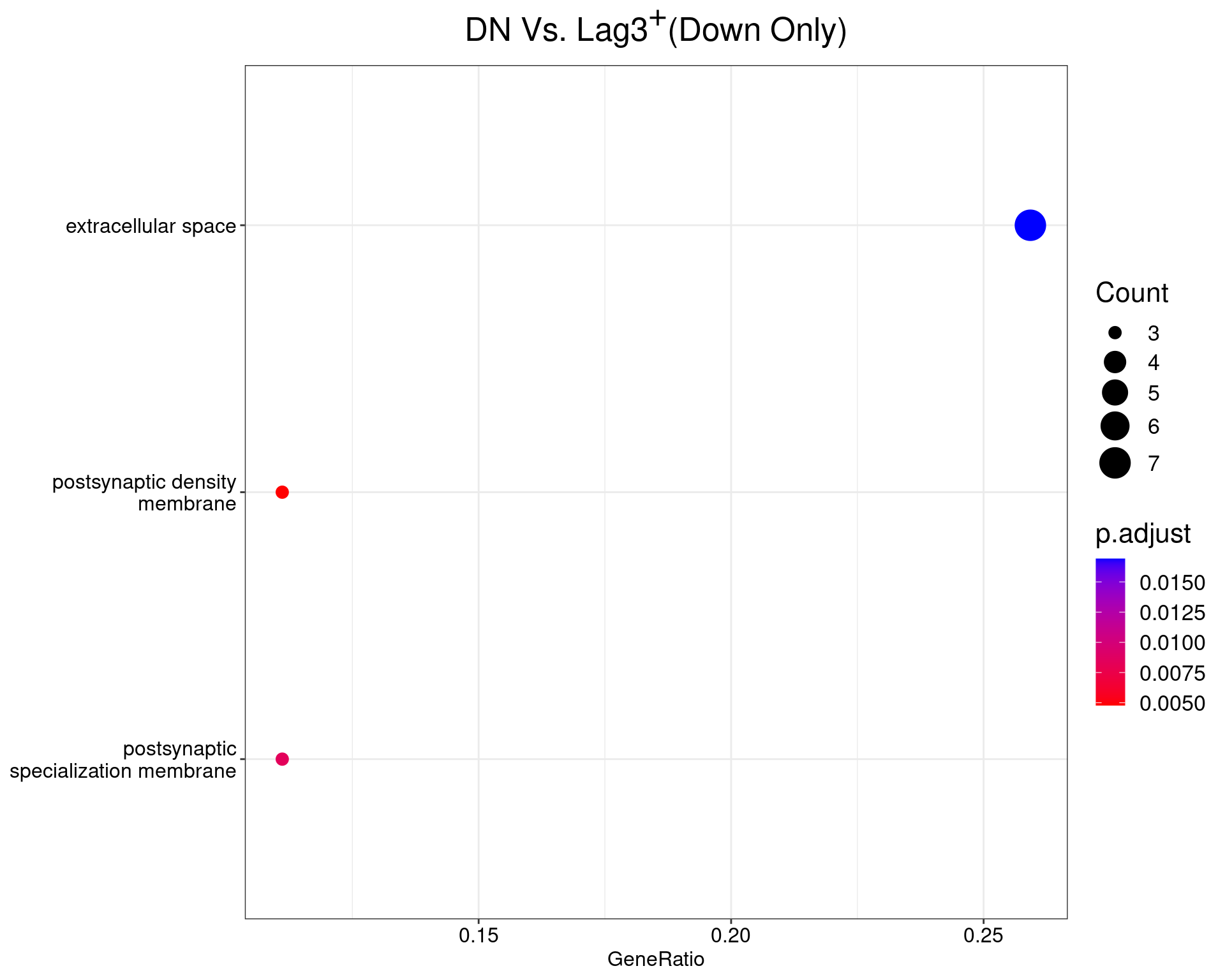
)Enrichment testing was repeated using all three available Gene
Ontologies and the function enrichGO() from the package
clusterProfiler. Ontologies were only considered to be
enriched amongst the down-regulated genes if a
Bonferroni-adjusted p-value < 0.05 was returned during enrichment
testing. Please note that a down-regulated gene does not always
correspond to an decrease in activity of a pathway.
DN Vs. Lag3+
dotplot(ego_results$DNvLAG3) +
  ggtitle(expression(paste("DN Vs. Lag", 3^{textstyle("+")}, "(Down Only)"))) +
  scale_y_discrete(labels = label_wrap(25)) +
  theme(
    plot.title = element_text(hjust = 0.5),
    text = element_text(size = 16)
  )
| Version | Author | Date |
|---|---|---|
| 0b3ca1b | steveped | 2022-11-17 |
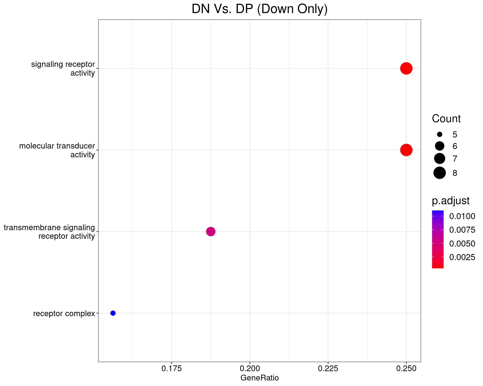
DN Vs. DP
dotplot(ego_results$DNvDP) +
  ggtitle("DN Vs. DP (Down Only)") +
  scale_y_discrete(labels = label_wrap(25)) +
  theme(
    plot.title = element_text(hjust = 0.5),
    text = element_text(size = 16)
  )
| Version | Author | Date |
|---|---|---|
| 0b3ca1b | steveped | 2022-11-17 |
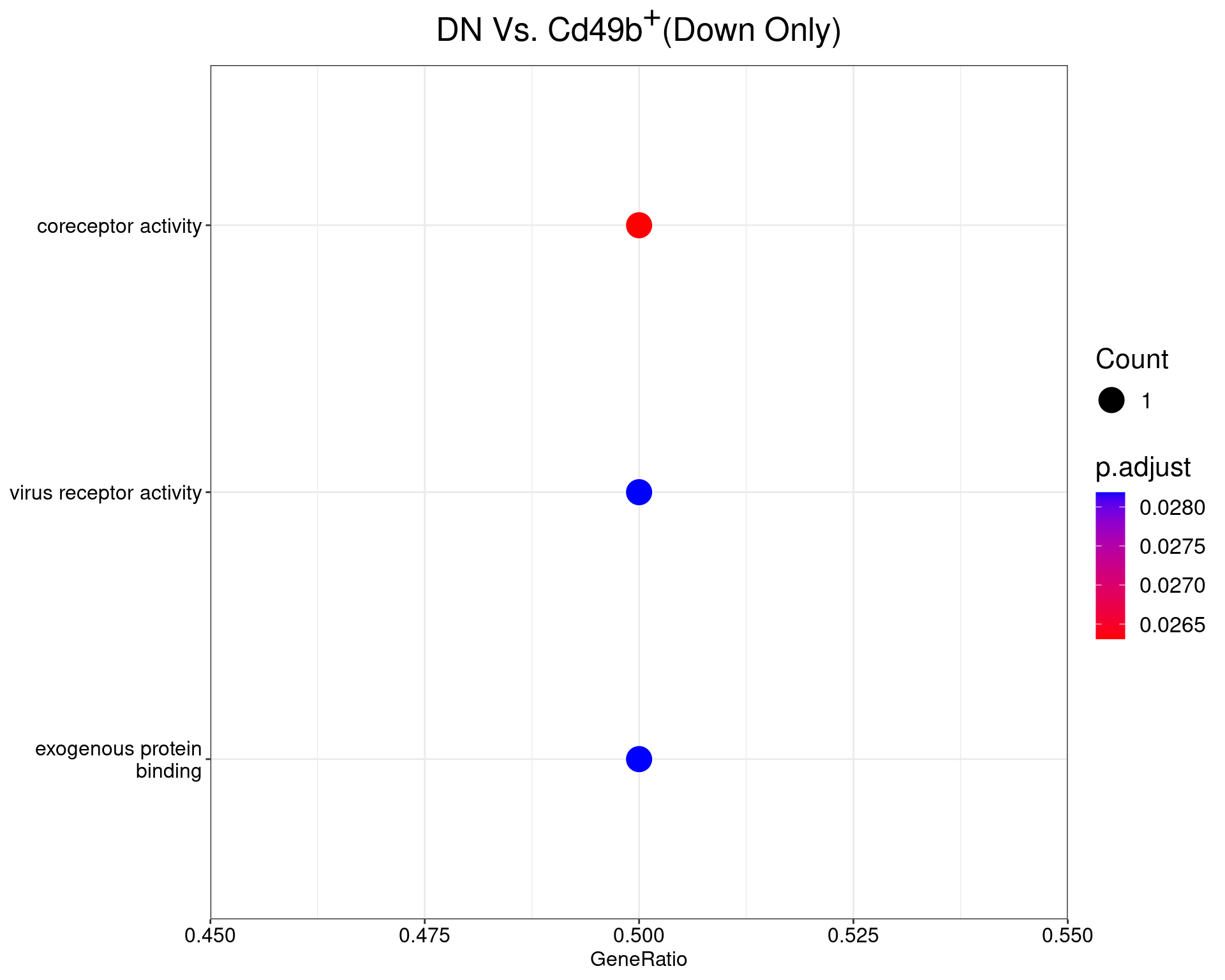
DN Vs. Cd49b+
dotplot(ego_results$DNvCD49b) +
  ggtitle(expression(paste("DN Vs. Cd49", b^{textstyle("+")}, "(Down Only)"))) +
  scale_y_discrete(labels = label_wrap(25)) +
  theme(
    plot.title = element_text(hjust = 0.5),
    text = element_text(size = 16)
  )
| Version | Author | Date |
|---|---|---|
| 0b3ca1b | steveped | 2022-11-17 |
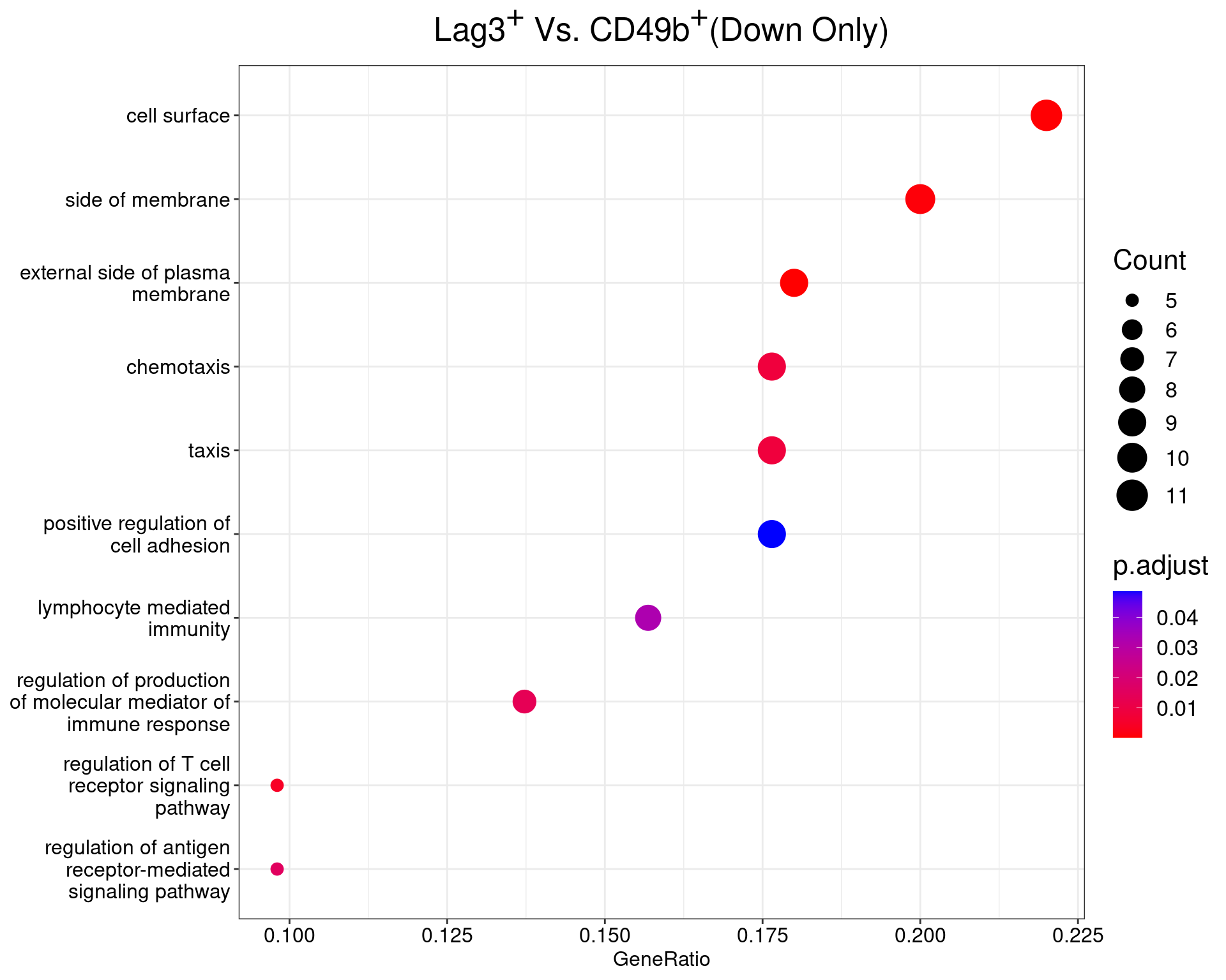
Lag3+ Vs Cd49+
dotplot(ego_results$LAG3vCD49b) +
  ggtitle(
    expression(
      paste("Lag", 3^{textstyle("+")}, " Vs. CD49", b^{textstyle("+")}, "(Down Only)")
    )
  ) +
  scale_y_discrete(labels = label_wrap(25)) +
  theme(
    plot.title = element_text(hjust = 0.5),
    text = element_text(size = 16)
  )
| Version | Author | Date |
|---|---|---|
| 0b3ca1b | steveped | 2022-11-17 |
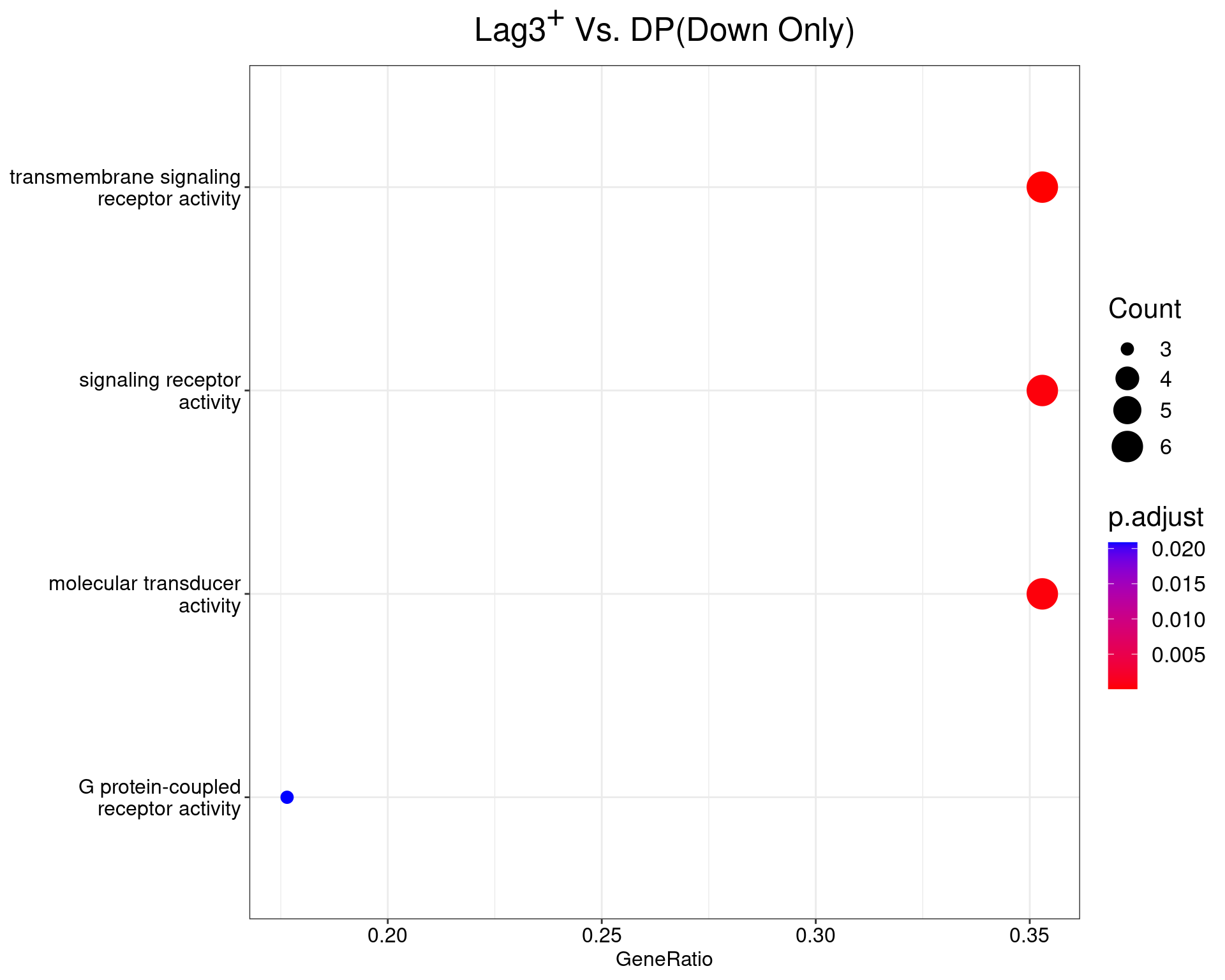
Lag3+ Vs. DP
dotplot(ego_results$LAG3vDP) +
  ggtitle(expression(paste("Lag", 3^{textstyle("+")}, " Vs. DP", "(Down Only)"))) +
  scale_y_discrete(labels = label_wrap(25)) +
  theme(
    plot.title = element_text(hjust = 0.5),
    text = element_text(size = 16)
  )
| Version | Author | Date |
|---|---|---|
| 0b3ca1b | steveped | 2022-11-17 |
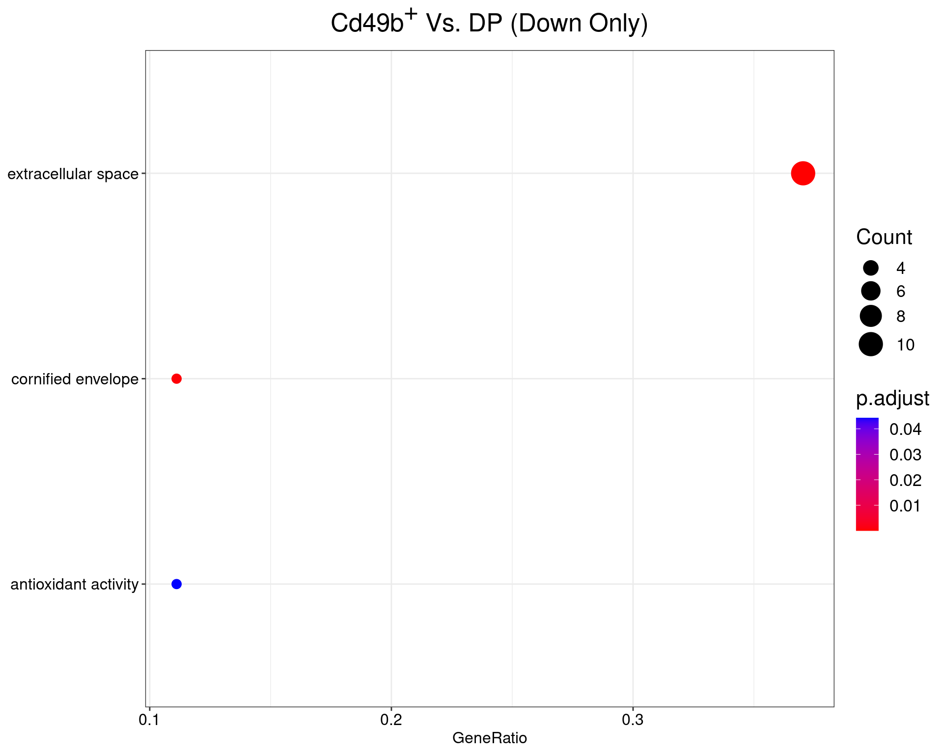
Cd49b+ Vs. DP
dotplot(ego_results$CD49bvDP) +
  ggtitle(expression(paste("Cd49", b^{textstyle("+")}, " Vs. DP (Down Only)"))) +
  scale_y_discrete(labels = label_wrap(25)) +
  theme(
    plot.title = element_text(hjust = 0.5),
    text = element_text(size = 16)
  )
| Version | Author | Date |
|---|---|---|
| 0b3ca1b | steveped | 2022-11-17 |
Enrichment Tables (Down Only)
ego_results <- ego_results[vapply(ego_results, nrow, integer(1)) > 0]
htmltools::tagList(
  names(ego_results) %>%
    lapply(
      function(x) {
        df <- ego_results[[x]] %>%
          as_tibble() %>%
          dplyr::filter(p.adjust < 0.05) %>%
          mutate(
            geneID = str_replace_all(geneID, "\\/", "; "),
            `% DE` = vapply(GeneRatio, function(x) eval(parse(text = x)), numeric(1)),
            `% BG` = vapply(BgRatio, function(x) eval(parse(text = x)), numeric(1))
          ) %>%
          dplyr::select(ONTOLOGY, ID, Description, Count, starts_with("%"), p.adjust, geneID) %>%
          arrange(p.adjust) %>%
          distinct(ONTOLOGY, geneID, .keep_all = TRUE)

        if (nrow(df)) {
          cp <- glue(
            "All {nrow(df)} ontologies considered enriched in the set of ",
            length(unique(unlist(dplyr::filter(top_tables[[x]], DE, logFC < -1)$entrezid))),
            " down-regulated genes mapped to EntrezIDs from the comparison {x}. Enrichment ",
            "testing was performed using Fisher's Exact Test compared to the set of ",
            comma(length(unique(universe))),
            " unique EntrezIDs mapped to genes considered as detectable. ",
            "The percentage of nonDE genes mapped to the ontology are also given. ",
            "P-values are Bonferroni adjusted and all pathways are considered enriched ",
            "using an adjusted p-value < 0.05. In order to see all DE genes, hover your ",
            "mouse over the final column. ",
            "Where the identical genes map to multiple terms within each ontology, only ",
            "the term with the lowest p-value (i.e. strongest enrichment) is shown. ",
            "As a result, some of the pathways seen in the above dotplots may not be ",
            "presented in these tables."
          )
          htmltools::div(
            htmltools::div(
              id = glue("{x}-down"),
              class="section level3",
              htmltools::h3(class = "tabset", x),
              htmltools::tags$em(cp),
              df %>%
                reactable(
                  filterable = TRUE,
                  columns = list(
                    ONTOLOGY = colDef(name = "Ontology", maxWidth = 100),
                    ID = colDef(name = "GO ID", maxWidth = 125),
                    Description = colDef(maxWidth = 250),
                    Count = colDef(name = "N<sub>DE</sub>", html = TRUE, maxWidth = 80),
                    `% DE` = colDef(format = colFormat(percent = TRUE, digits = 1), maxWidth = 85),
                    `% BG` = colDef(format = colFormat(percent = TRUE, digits = 1), maxWidth = 85),
                    p.adjust = colDef(
                      name = "p<sub>adj</sub>", html = TRUE, maxWidth = 100,
                      cell = function(value) {
                        fm <- ifelse(value < 0.001, "%.2e", "%.3f")
                        sprintf(fm, value)
                      }
                    ),
                    geneID = colDef(
                      name = "DE Genes",
                      cell = function(value) with_tooltip(value, width = 100)
                    )
                  )
                )
            )
          )
        } else {
          cat(glue("No enrichment was found for {x}\n\n"))
        }
      }
    )
)
DNvLAG3
All 2 ontologies considered enriched in the set of 29 down-regulated genes mapped to EntrezIDs from the comparison DNvLAG3. Enrichment testing was performed using Fisher's Exact Test compared to the set of 10,006 unique EntrezIDs mapped to genes considered as detectable. The percentage of nonDE genes mapped to the ontology are also given. P-values are Bonferroni adjusted and all pathways are considered enriched using an adjusted p-value < 0.05. In order to see all DE genes, hover your mouse over the final column. Where the identical genes map to multiple terms within each ontology, only the term with the lowest p-value (i.e. strongest enrichment) is shown. As a result, some of the pathways seen in the above dotplots may not be presented in these tables.DNvDP
All 3 ontologies considered enriched in the set of 33 down-regulated genes mapped to EntrezIDs from the comparison DNvDP. Enrichment testing was performed using Fisher's Exact Test compared to the set of 10,006 unique EntrezIDs mapped to genes considered as detectable. The percentage of nonDE genes mapped to the ontology are also given. P-values are Bonferroni adjusted and all pathways are considered enriched using an adjusted p-value < 0.05. In order to see all DE genes, hover your mouse over the final column. Where the identical genes map to multiple terms within each ontology, only the term with the lowest p-value (i.e. strongest enrichment) is shown. As a result, some of the pathways seen in the above dotplots may not be presented in these tables.DNvCD49b
All 1 ontologies considered enriched in the set of 2 down-regulated genes mapped to EntrezIDs from the comparison DNvCD49b. Enrichment testing was performed using Fisher's Exact Test compared to the set of 10,006 unique EntrezIDs mapped to genes considered as detectable. The percentage of nonDE genes mapped to the ontology are also given. P-values are Bonferroni adjusted and all pathways are considered enriched using an adjusted p-value < 0.05. In order to see all DE genes, hover your mouse over the final column. Where the identical genes map to multiple terms within each ontology, only the term with the lowest p-value (i.e. strongest enrichment) is shown. As a result, some of the pathways seen in the above dotplots may not be presented in these tables.LAG3vCD49b
All 14 ontologies considered enriched in the set of 53 down-regulated genes mapped to EntrezIDs from the comparison LAG3vCD49b. Enrichment testing was performed using Fisher's Exact Test compared to the set of 10,006 unique EntrezIDs mapped to genes considered as detectable. The percentage of nonDE genes mapped to the ontology are also given. P-values are Bonferroni adjusted and all pathways are considered enriched using an adjusted p-value < 0.05. In order to see all DE genes, hover your mouse over the final column. Where the identical genes map to multiple terms within each ontology, only the term with the lowest p-value (i.e. strongest enrichment) is shown. As a result, some of the pathways seen in the above dotplots may not be presented in these tables.CD49bvDP
All 3 ontologies considered enriched in the set of 28 down-regulated genes mapped to EntrezIDs from the comparison CD49bvDP. Enrichment testing was performed using Fisher's Exact Test compared to the set of 10,006 unique EntrezIDs mapped to genes considered as detectable. The percentage of nonDE genes mapped to the ontology are also given. P-values are Bonferroni adjusted and all pathways are considered enriched using an adjusted p-value < 0.05. In order to see all DE genes, hover your mouse over the final column. Where the identical genes map to multiple terms within each ontology, only the term with the lowest p-value (i.e. strongest enrichment) is shown. As a result, some of the pathways seen in the above dotplots may not be presented in these tables.LAG3vDP
All 2 ontologies considered enriched in the set of 17 down-regulated genes mapped to EntrezIDs from the comparison LAG3vDP. Enrichment testing was performed using Fisher's Exact Test compared to the set of 10,006 unique EntrezIDs mapped to genes considered as detectable. The percentage of nonDE genes mapped to the ontology are also given. P-values are Bonferroni adjusted and all pathways are considered enriched using an adjusted p-value < 0.05. In order to see all DE genes, hover your mouse over the final column. Where the identical genes map to multiple terms within each ontology, only the term with the lowest p-value (i.e. strongest enrichment) is shown. As a result, some of the pathways seen in the above dotplots may not be presented in these tables.
sessionInfo()R version 4.3.0 (2023-04-21)
Platform: x86_64-pc-linux-gnu (64-bit)
Running under: Ubuntu 20.04.6 LTS
Matrix products: default
BLAS: /usr/lib/x86_64-linux-gnu/blas/libblas.so.3.9.0
LAPACK: /usr/lib/x86_64-linux-gnu/lapack/liblapack.so.3.9.0
locale:
[1] LC_CTYPE=en_AU.UTF-8 LC_NUMERIC=C
[3] LC_TIME=en_AU.UTF-8 LC_COLLATE=en_AU.UTF-8
[5] LC_MONETARY=en_AU.UTF-8 LC_MESSAGES=en_AU.UTF-8
[7] LC_PAPER=en_AU.UTF-8 LC_NAME=C
[9] LC_ADDRESS=C LC_TELEPHONE=C
[11] LC_MEASUREMENT=en_AU.UTF-8 LC_IDENTIFICATION=C
time zone: Australia/Adelaide
tzcode source: system (glibc)
attached base packages:
[1] stats4 stats graphics grDevices utils datasets methods
[8] base
other attached packages:
[1] scales_1.2.1 glue_1.6.2 htmltools_0.5.5
[4] reactable_0.4.4 org.Mm.eg.db_3.17.0 AnnotationDbi_1.62.0
[7] IRanges_2.34.0 S4Vectors_0.38.0 Biobase_2.60.0
[10] BiocGenerics_0.46.0 clusterProfiler_4.8.0 magrittr_2.0.3
[13] pheatmap_1.0.12 RColorBrewer_1.1-3 edgeR_3.42.0
[16] limma_3.56.0 lubridate_1.9.2 forcats_1.0.0
[19] stringr_1.5.0 dplyr_1.1.2 purrr_1.0.1
[22] readr_2.1.4 tidyr_1.3.0 tibble_3.2.1
[25] ggplot2_3.4.2 tidyverse_2.0.0 workflowr_1.7.0
loaded via a namespace (and not attached):
[1] rstudioapi_0.14 jsonlite_1.8.4 farver_2.1.1
[4] rmarkdown_2.21 fs_1.6.2 zlibbioc_1.46.0
[7] vctrs_0.6.2 memoise_2.0.1 RCurl_1.98-1.12
[10] ggtree_3.8.0 gridGraphics_0.5-1 sass_0.4.5
[13] bslib_0.4.2 htmlwidgets_1.6.2 plyr_1.8.8
[16] cachem_1.0.7 whisker_0.4.1 igraph_1.4.2
[19] lifecycle_1.0.3 pkgconfig_2.0.3 gson_0.1.0
[22] Matrix_1.5-4 R6_2.5.1 fastmap_1.1.1
[25] GenomeInfoDbData_1.2.10 digest_0.6.31 aplot_0.1.10
[28] enrichplot_1.20.0 colorspace_2.1-0 patchwork_1.1.2
[31] ps_1.7.5 rprojroot_2.0.3 crosstalk_1.2.0
[34] RSQLite_2.3.1 reactR_0.4.4 labeling_0.4.2
[37] fansi_1.0.4 timechange_0.2.0 httr_1.4.5
[40] polyclip_1.10-4 compiler_4.3.0 here_1.0.1
[43] bit64_4.0.5 withr_2.5.0 downloader_0.4
[46] BiocParallel_1.34.0 viridis_0.6.2 DBI_1.1.3
[49] highr_0.10 ggforce_0.4.1 MASS_7.3-59
[52] HDO.db_0.99.1 tools_4.3.0 scatterpie_0.1.9
[55] ape_5.7-1 httpuv_1.6.9 callr_3.7.3
[58] nlme_3.1-162 GOSemSim_2.26.0 promises_1.2.0.1
[61] shadowtext_0.1.2 grid_4.3.0 getPass_0.2-2
[64] reshape2_1.4.4 fgsea_1.26.0 generics_0.1.3
[67] gtable_0.3.3 tzdb_0.3.0 data.table_1.14.8
[70] hms_1.1.3 tidygraph_1.2.3 utf8_1.2.3
[73] XVector_0.40.0 ggrepel_0.9.3 pillar_1.9.0
[76] yulab.utils_0.0.6 later_1.3.0 splines_4.3.0
[79] tweenr_2.0.2 treeio_1.24.0 lattice_0.21-8
[82] bit_4.0.5 tidyselect_1.2.0 GO.db_3.17.0
[85] locfit_1.5-9.7 Biostrings_2.68.0 knitr_1.42
[88] git2r_0.32.0 gridExtra_2.3 xfun_0.39
[91] graphlayouts_0.8.4 stringi_1.7.12 lazyeval_0.2.2
[94] ggfun_0.0.9 yaml_2.3.7 evaluate_0.20
[97] codetools_0.2-19 ggraph_2.1.0 qvalue_2.32.0
[100] ggplotify_0.1.0 cli_3.6.1 munsell_0.5.0
[103] processx_3.8.1 jquerylib_0.1.4 Rcpp_1.0.10
[106] GenomeInfoDb_1.36.0 png_0.1-8 parallel_4.3.0
[109] ellipsis_0.3.2 blob_1.2.4 DOSE_3.26.0
[112] bitops_1.0-7 tidytree_0.4.2 viridisLite_0.4.1
[115] crayon_1.5.2 rlang_1.1.0 cowplot_1.1.1
[118] fastmatch_1.1-3 KEGGREST_1.40.0